Excel to the end of a column

Most of us work with tabular data in Excel where the data is arranged in columns.

And one of the common tasks most Excel users have to do is to go to the end of the data in the column (i.e., the last filled cell).

While you can quickly go to the end of the column to the last filled cell, or select the entire column till the last filled cell with an easy keyboard shortcut, things can get a bit complicated if you have blank cells in the column.

In this tutorial, I will show you a couple of simple methods (including keyboard shortcuts) that you can use to quickly select the end of the column in Excel.

The method you choose would depend on how your data is structured, and I’ll make sure to mention the pros and cons of each method that I covered in this tutorial.

Keyboard Shortcut to Select the End of the Column (CONTROL + SHIFT + Arrow Key)

Below, I have a data set where I have the items in column A and I have the expenses made every day in column B, and I want to select all the expense values in column B.

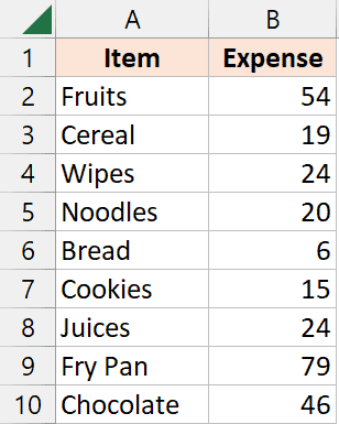
If your data set has no blank cells in any of the cells in the column, you can easily select till the end of the column by using the below keyboard shortcut:

Control + Shift + Down Arrow Key

To use the above keyboard shortcut:

1. Select the first cell that you want to be a part of the selection (cell B2 in this example)

1. Hold the Control key and the Shift key (together)
2. With the Control and  Shift key pressed, press the down arrow key once

With the above keyboard shortcut, Excel would magically start the selection from the first selected cell and extend it till the last filled cell in the column.

But life ain’t perfect, and the same can be said for your data in Excel.

Often, data in columns have blank cells that can complicate selecting the entire column till the last filled cell.

When there are Blank Cells in the Column

Below I have the same data set but there are some blank cells in column B, and I want to start with cell B2 and select till the end of the data in the column.

With this data set, if you try and use the above keyboard shortcut, you would notice that the selection is made only till the cell before the first empty cell.

So we need to use the same keyboard shortcut a little differently.

Below are the steps to select till the end of the data in a column when you have blank cells in the column:

1. Select the first cell from which you want the selection to begin (cell B2 in our example)
2. Hold the Control and the Shift key
3. Press the down arrow key, and keep it pressed
4. Once you have reached the end of the column in the worksheet, press the up arrow key (while still holding the Control and the Shift key)

While this is not the most elegant solution, it gets the work done, and if you do not have a lot of blank cells in your column, it could be quite fast.

One scenario where this may not be the best method to use is when you have a lot of blank cells (say a blank cell in every other row or after every two or three rows). While the method would still work in such a scenario, it could take a few more seconds (which in my experience is not something most Excel users are willing to give).

Also read: Select Every Other Row in Excel

Keyboard Shortcut to Select the End of the Column (CONTROL + SHIFT + End)

Below, I have a data set where I want to select all the expense values in column B.

Here is another keyboard shortcut that you can use to select the end of the data in a column:

Control + Shift + End

Below are the steps to use this keyboard shortcut:

1. Select the first cell from which you want the selection to begin (cell B2 in our example)
2. Hold the Control and the Shift key
3. Press the End key

The above steps would start the selection from cell B2, and select all the cells till the last used cell.

In most cases, the last cell in your column would also be the last used cell, so this keyboard shortcut should work perfectly in selecting the end of the data in the column.

And the great thing about this method is that you do not need to worry about blank cells, as it selects all the cells between the first selected cell and the last used cell.

When You Have More Data On the Right

When you use Control + Shift + End, it starts the selection from the cell that you selected (B2 in our example), and extends the selection till the last cell in the used range.

So if you have more data on the right of the column, using the above keyboard shortcut would not only select the existing column but also any data that Is to the right,

And sometimes, the used range would remain in the memory of Excel even if you have deleted that data. For example, if I enter some value in the cell E20 and then delete it, the used range in excel would be A1:E20 (as E20 is the last used cell in the memory of Excel).

So there is a possibility that when you use the above keyboard shortcut, it selects more cells on the right and below the column that we intend to select.

In such a scenario, you can use the same keyboard shortcuts with a minor twist:

1. Select the first cell from which you want the selection to begin (cell B2 in our example)
2. Hold the Control and the Shift key
3. Press the End key
4. If additional blank rows and columns have been selected, keep the Control and Shift keys pressed, press the Left key once, and then press the Up arrow key once
5. Hold the Shift key and keep pressing the left arrow key till only the column that you need is selected.

While this is not the most elegant solution, when you get used to it, you will find it faster than manually selecting a column till the end of the data.

Using the Name Box

Name Box allows you to quickly select a range of cells by entering the reference in the name box.

You will find the name box on the left of the formula bar, just below the formula bar.

Let’s say that I want to select column A (starting from cell A2) till the last filled cell, where I have blank cells in the column (which will make using the keyboard shortcut Control + Shift + Down arrow key challenging).

Below are the steps to use the name box to select the entire column A till the end of the data (i.e., till the last filled cell):

1. Place the cursor in the Name Box
2. Enter the below cell reference in the Name Box – A2:A1048576

1. Hit the Enter key. This will select all the cells in the specified range
2. Hold the Control and the Shift key and then press the Up-arrow key.

The above steps would select all the cells in column A till the last filled cell.

Note: This method works in Google Sheets as well (you can use the exact same steps)

Using Go To Dialog Box

Just like the Name Box, you can also use the Go To dialog box to quickly select a range of cells by specifying the reference of that range

Let’s say I want to select the range B2:B100.

Below are the steps to do this using the Go To dialog box

1. Go to the worksheet where you want to select this range
2. Press the F5 key on your keyboard. This will open the Go-To dialog box

1. Enter the below cell reference in the Reference field

B2:B100

1. Click OK

There were steps that would instantly select the range that you specified in the Go-To dialog box.

So these are some of the shortcut ways you can use to quickly select data in a column till the end of the data.

While the methods I’ve covered here have been shown using data in a column, you can use the same methods to select data till the end of the rows as well

While you always have the option to do this manually using the mouse, if you need to do this quite often, knowing these shortcuts will significantly improve your efficiency.

Other Excel articles you may also like:

• 7 Easy Ways to Select Multiple Cells in Excel
• How to Select Non-adjacent cells in Excel? (4 Easy Ways)
• How to Deselect Cells in Excel (An Easy Way)
• [Quick Tip] How to Select 500 cells/rows in Excel (with a single click)
• 3 Quick Ways to Select Visible Cells in Excel
• How to Select Every Third Row in Excel (or select every Nth Row)
• How to Quickly Select a Far-off Excel Cell or Range

There may be instances where you need to add the same text to all cells in a column. You might need to add a particular title before names in a list, or a particular symbol at the end of the text in every cell.

The good thing is you don’t need to do this manually.

Excel provides some really simple ways in which you can add text to the beginning and/ or end of the text in a range of cells.

In this tutorial we will see 4 ways to do this:

• Using the ampersand operator (&)
• Using the CONCATENATE function
• Using the Flash Fill feature
• Using VBA

So let’s get started!

Method 1: Using the ampersand Operator

An ampersand (&) can be used to easily combine text strings in Excel. Let’s see how you use it to add text at the beginning or end or both in Excel.

Using the ampersand Operator to Add Text to the Beginning of all Cells

The ampersand (&) is an operator that is mainly used to join several text strings into one.

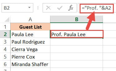
Here’s how you can use it to add text to the beginning of all cells in a range. Let us assume you have the following list of names and want to add the title “Prof.” before every name:

Below are the  steps to add  a text before a text string in Excel:

1. Click on the first cell of the column where you want the converted names to appear (B2).
2. Type equal sign (=), followed by the text “Prof. “, followed by an ampersand (&).
3. Select the cell containing the first name (A2).
4. Press the Return Key.
5. You will notice that the title “Prof.” is added before the first name in the list.
6. It’s now time to copy this formula to the rest of the cells in the column. Simply double click the fill handle (located at the bottom right of cell B2). Alternatively, you can drag down the fill handle to achieve the same effect.

That’s it, all your cells in column B should now contain the title “Prof.” preceding each name.

Using the ampersand Operator to Add Text to the End of all Cells

Now let us see how to add some text to the end of every name in the dataset. Let us say you want to add the text “(MD)” at the end of every name. In that case, here are the steps you need to follow:

1. Click on the first cell of the column where you want the converted names to appear (C2 in our case).
2. Type equal sign (=)
3. Select the cell containing the first name (B2 in our case).
4. Next, insert an ampersand (&), followed by the text “ (MD)”.
5. Press the Return Key.
6. You will notice that the text “(MD).” added after the first name in the list.
7. It’s now time to copy this formula to the rest of the cells in the column. Simply double click the fill handle (located at the bottom right of cell C2). Alternatively, you can drag down the fill handle to achieve the same effect.

All your cells in column C should now contain the text “(MD”) at the end of each name.

Method 2: Using the CONCATENATE Function

CONCATENATE is an Excel function that you can use to add text at the beginning and end of the text string.

Let’s see how to use CONCATENATE to do this.

Using CONCATENATE to Add Text to the Beginning of all Cells

The CONCATENATE() function provides the same functionality as the ampersand (&) operator. The only difference is in the way both are used.

The general syntax for the CONCATENATE function is:

=CONCATENATE(text1, [text2], …)

Where text1, text2, etc. are substrings that you want to combine together.

Let’s apply the CONCATENATE function to the same dataset as above:

1. Click on the first cell of the column where you want the converted names to appear (B2).
2. Type equal sign (=).
3. Enter the function CONCATENATE, followed by an opening bracket (.
4. Type the title “Prof. ” in double-quotes, followed by a comma (,).
5. Select the cell containing the first name (A2)
6. Place a closing bracket. In our example, your formula should now be: =CONCATENATE(“Prof. “,A2).
7. Press the Return Key.
8. You will notice that the title “Prof.” is added before the first name on the list.
9. It’s now time to copy this formula to the rest of the cells in the column. Simply double click the fill handle (located at the bottom right of cell B2). Alternatively, you can drag down the fill handle to achieve the same effect.

That’s it, all your cells in column B should now contain the title “Prof.” preceding each name.

Using CONCATENATE to Add Text to the End of all Cells

Now let us see how to add some text to the end of every name in the dataset. Let us say you want to add the text “(MD)” at the end of every name. In that case, here are the steps you need to follow:

1. Click on the first cell of the column where you want the converted names to appear (C2 in our example).
2. Type equal sign (=).
3. Enter the function CONCATENATE, followed by an opening bracket (.
4. Select the cell containing the first name (B2 in our example).
5. Next, insert a comma, followed by the text “ (MD)”.
6. Place a closing bracket. In our example, your formula should now be: =CONCATENATE(B2,” (MD)”).
7. Press the Return Key.
8. You will notice that the text “(MD).” added after the first name in the list.
9. It’s now time to copy this formula to the rest of the cells in the column. Simply double click the fill handle (located at the bottom right of cell C2).

All your cells in column C should now contain the text “(MD”) at the end of each name.

Notice that since you’re using a formula, your column C depends on columns A and B. So if you make any changes to the original values in column A, they get reflected in column C.

If you decide to only retain the converted names and delete columns A and B, you will get an error, as shown below:

To make sure that this does not happen, it’s best to first convert the formula results to permanent values copying them and pasting them as values in the same column (Right-click and select Paste Options->Values from the Popup menu).

Now you can go ahead and delete columns A and B if you need to.

Also read: How to Remove First Character in Excel?

Method 3: Using the Flash Fill Feature

Flash fill is a relatively new feature that looks at the pattern of what you are trying to achieve and then does it for all the cells in a column.

You can also use Flash fill to so text manipulation as we will see in the following examples.

Using Flash Fill to Add Text to the Beginning of all Cells

The Excel flash fill feature is like a magical button. It is available if you’re on any Excel version from 2013 onwards.

The feature takes advantage of Excel’s pattern recognition capabilities. It basically recognizes a pattern in your data and automatically fills in the other cells of the column with the same pattern for you.

Here’s how you can use Flash Fill to add text to the beginning of all cells in a column:

1. Click on the first cell of the column where you want the converted names to appear (B2).
2. Manually type in the text Prof. , followed by the first name of your list.
3. Press the Return Key.
4. Click on cell B2 again.
5. Under the Data tab, click on the Flash Fill button (in the ‘Data Tools’ group). Alternatively, you can just press CTRL+E on your keyboard (Command+E if you’re on a Mac).

This will copy the same pattern to the rest of the cells in the column… in a flash!

Using Flash Fill to Add Text to the End of all Cells in a Column

If you want to add the text “ (MD)” to the end of the names, follow the same steps:

1. Click on the first cell of the column where you want the converted names to appear (C2).
2. Manually type in or copy the text from column B2 into C2.
3. Add the text “(MD)” after that.
4. Under the Data tab, click on the Flash Fill or press CTRL+E on your keyboard (Command+E if you’re on a Mac).

That’s all, you get every cell filled in with the same pattern!

We especially like this method because it is simple, quick, and easy. Moreover, since it’s formula-free, the results do not depend on the original columns.

So they remain unchanged even if you delete rows A and B!

Method 4: Using VBA Code

And of course, if you’re comfortable with VBA, you can also add text before or after a text string using it.

Using VBA to Add Text to the Beginning of all Cells in a Column

If coding with VBA does not intimidate you then this method can help get your work done quickly too.

Here’s the code we will be using to add the title “Prof. “ to the beginning of all cells in a range. You can select and copy it:

Sub add_text_to_beginning()
Dim rng As Range
Dim cell As Range
Set rng = Application.Selection
For Each cell In rng
cell.Offset(0, 1).Value = "Prof. " & cell.Value
Next cell
End Sub

Follow these steps to use the above code:

1. From the Developer Menu Ribbon, select Visual Basic.
2. Once your VBA window opens, Click Insert->Module. Now you can start coding. Type or copy-paste the above lines of code into the module window. Your code is now ready to run.
3. Select the range of cells containing the text you want to convert. Make sure the column next to it is blank because this is where the code will display the results.
4. Navigate to Developer->Macros-> add_text_to_beginning->Run.

You will now see the converted text next to your selected range of cells.

Note: You can change the text in line 6 from “Prof. ” to whatever text you need to add to the beginning of all cells.

Using VBA to Add Text to the End of all Cells in a Column

Now, what if you want to add text to the end of all the cells, instead of the beginning? This only involves making a tweak to line 6 of the above code. So if you want to add the text “ (MD)” to the end of all cells, change line 6 to:

cell.Offset(0, 1).Value = cell.Value & “ (MD)”

So your full code should now be:

Sub add_text_to_end()
Dim rng As Range
Dim cell As Range
Set rng = Application.Selection
For Each cell In rng
cell.Offset(0, 1).Value = cell.Value & " (MD)"
Next cell
End Sub

Here’s the final result:

You can now delete the first two columns if you need to. Do remember to keep a backup of your sheet, because the results of VBA code are usually irreversible.

Note: You can change the text in line 6 from “ (MD)” to whatever text you need to add to the end of all cells in the range.

In this tutorial, we showed you four ways in which you can add text to the beginning and/ or end of all cells in a range.

There are plenty of other methods that you can find online too, and all of them work just as well as the ones shown here.

You may feel free to choose whatever method suits you, your requirement, and your version of Excel. In the end, what matters is getting what you need to be done quickly and effectively.

Other Excel tutorials you may like:

• How to Remove Text after a Specific Character in Excel
• How to Reverse a Text String in Excel
• How to Count How Many Times a Word Appears in Excel
• How to Remove Commas in Excel (from Numbers or Text String)
• How to Remove a Specific Character from a String in Excel
• How to Change Uppercase to Lowercase in Excel
• How to Separate Address in Excel?
• How to Concatenate with Line Breaks in Excel?
• How to Separate Names in Excel

Sometimes we need to select the column but only the used range, instead of the whole column.

We can do it with mouse if the data size if not so big.

However, using a mouse could be really time-consuming when you have thousands of rows on your Excel sheets. It can really piss one off if one accidentally release one’s finger when selecting the cells.

In this article, I am going to show you how to select column to end of data. The same concept applies to rows. I will provide you with 4 ways to deal with different situations.

Comparison (4 ways)

I will be showing you 4 ways to select to end of column from a cell. Here I want you to take a look at the comparison table.

Each method has its edges and drawbacks. You can pick one that is most suitable for you.

If you are keen to learn, I suggest you memorising all this.

Method	Edge	Drawback
Ctrl Shift Arrow	Time-efficient when the range is contiguous	Time-consuming if there are too many empty cells within the data
Ctrl End	No need to guess the last row	Time-consuming if there are too many empty cells within the data
Go To	Time-efficient when the range is non-contiguous	Need to estimate how many rows there are
VBA	Almost always fastest once created	Take time to create the script

Example

In this article, I will be illustrating how to select columns/rows to the end of the data by this example.

Most of you may have learnt that the shortcut key to select columns to the end of data is Ctrl + Shift + down arrow.

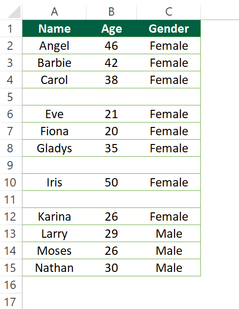
I would like to add some complexity to the situation by adding some blank cells in between different rows.

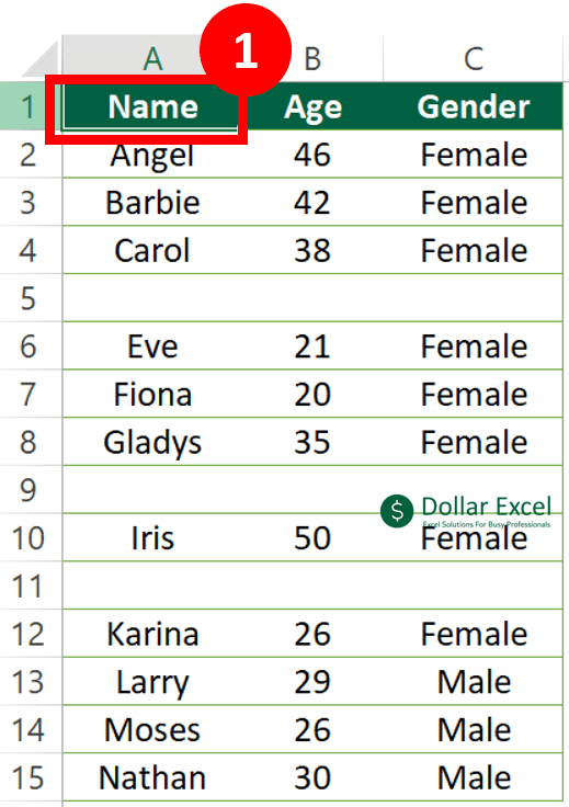
As you can see, the end of column A is Cell A15.

In Cell A1 to Cell A15, there are a couples of empty cells, which means the data is not contiguous.

Sample Workbook

Here is a Excel document you can interact with. You can play with it a bit to practise the trick.

Download the workbook to practice it by yourself!

Expected Outcome

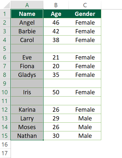
We would like to select Column A to the end of the data (Cell A15).

1. Select column to end of data by Ctrl Shift Arrow

Step 1: Select your starting cell

Step 2: Press Ctrl + Shift + down arrow (don’t release any of them)

In the Gif, I am pressing down arrow one at a time to show you how it works.

When you actually use it, you can keep pressing the down arrow key and release it once you find the last row.

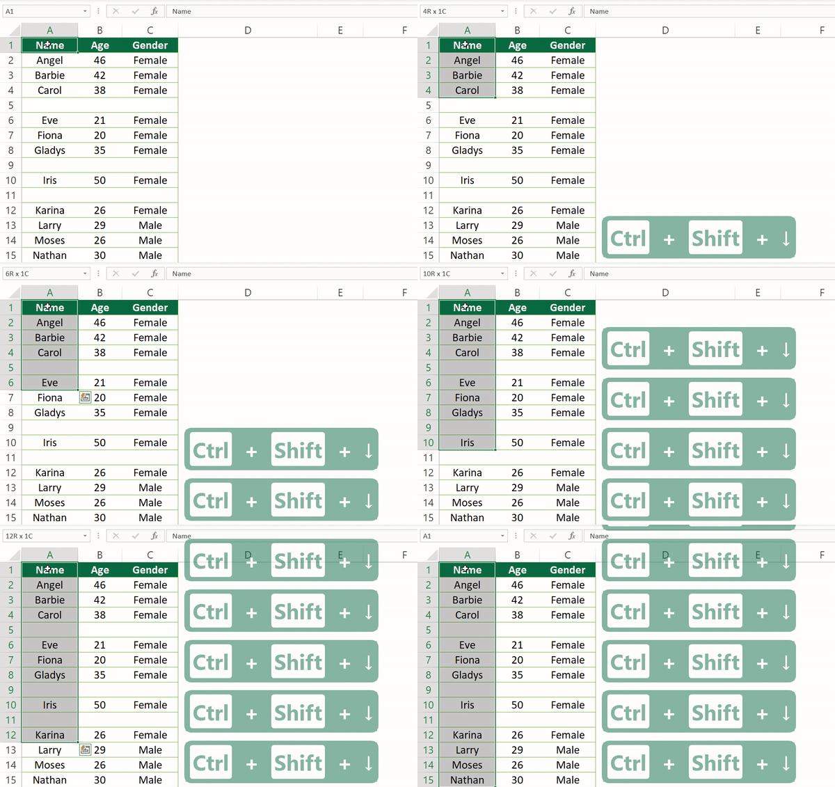
Step 3: Release all 3 keys after you select the range to the end of data

You are done.

The first method is the most straightforward one. All you need to do is just repeating the normal shortcut key.

2. Select column to end of data by Ctrl End

This one is a variation of option 1.

The concept is similar to option 1 but it is slightly different.

Step 1: Press Ctrl End

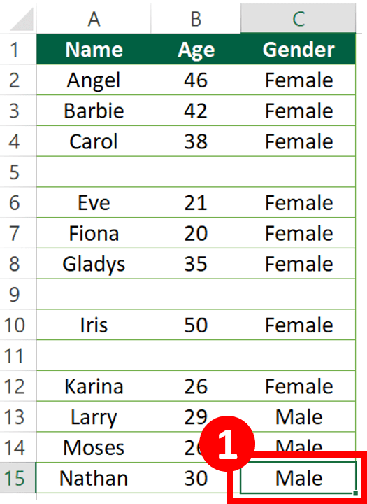
Step 2: Press Ctrl + Left Arrow until you reached Column A

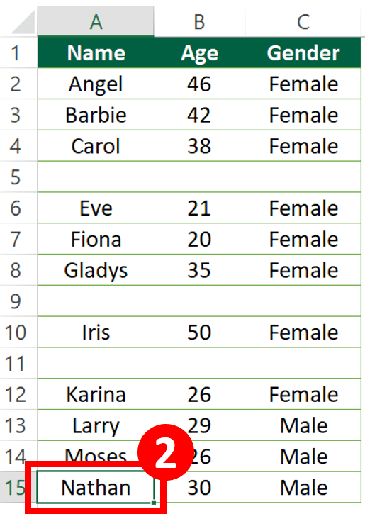
Step 3: Press Ctrl + Shift + Up Arrow until you reached your starting cell

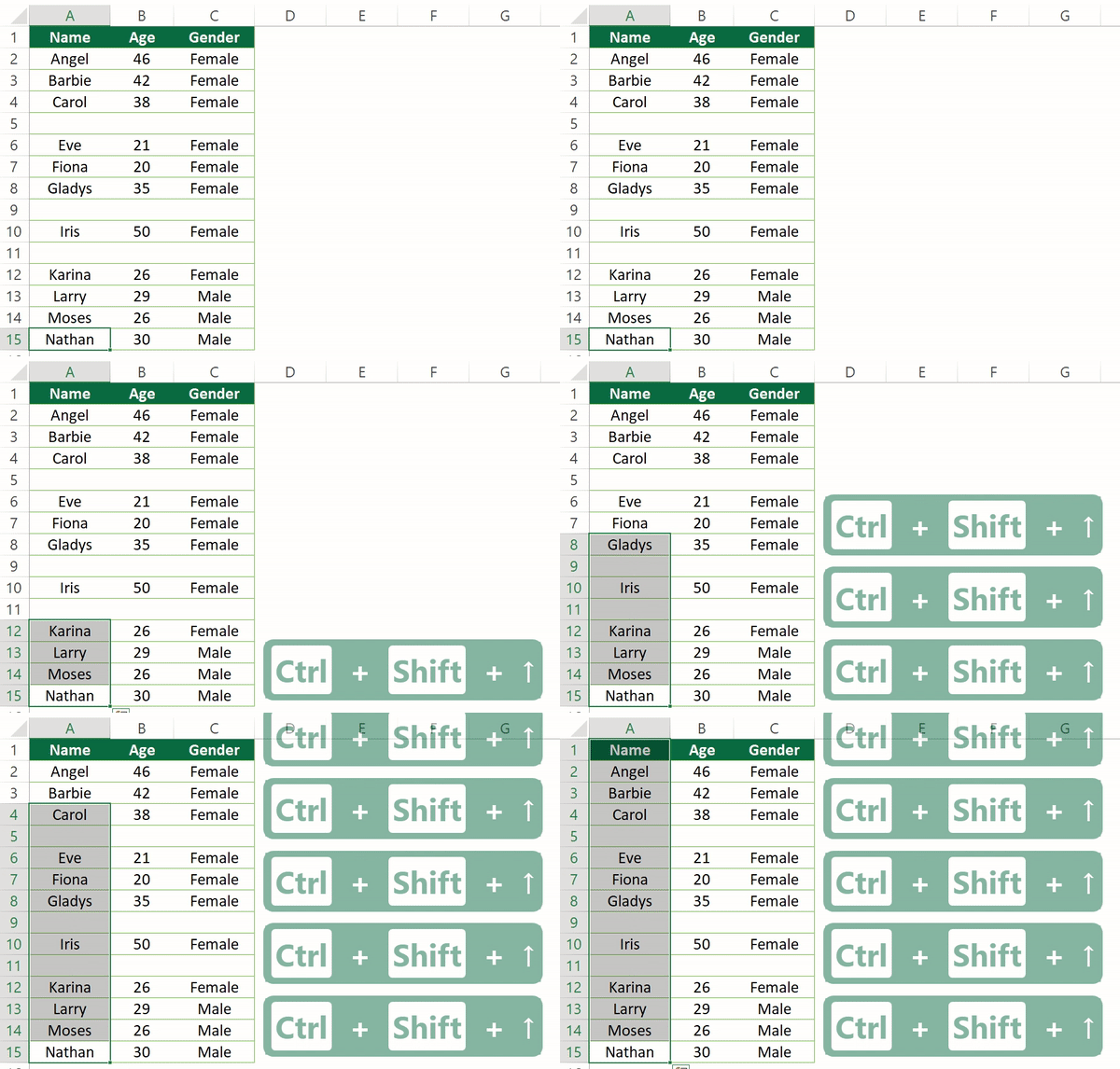
You may consider the option 2 a bit redundant since we already have option 1.

I will tell you why it is not.

When we are using option 1, we cannot press the Ctrl + Shift + down arrow too fast since we are usually unsure of where is the end of the column.

On the contrary, we can keep pressing the Ctrl + Shift + up arrow without releasing it when using the option 1. This is because usually the start of the column is cell A1.

That is why option 2 comes in more handy in most of the time.

3. Select column to end of data by Go To

Step 1: Spot the last cell in the column

You don’t need to select the cell. You just need to know which cell is the last cell in the column.

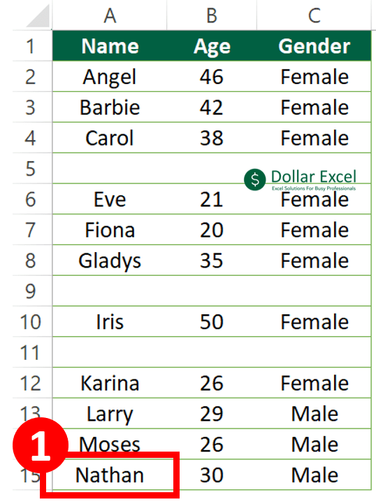
Step 2: Press Ctrl + G to open the “Go To” dialog

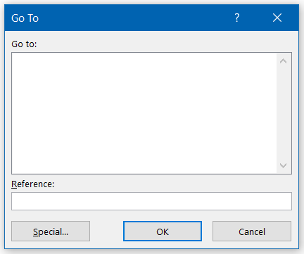
Step 3-4: Type the cell range into the reference box and press “OK”

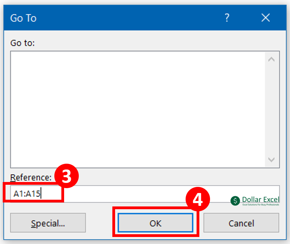
You have reached the end of the column at a few keystrokes. Now you can repeat the ctrl + shift + up arrow.

You may wonder why we would use this Go to dialog when we already have Ctrl + End.

This is because Go to dialog actually gives you greater flexibility.

With Ctrl End, the last cell used in the current Excel worksheet is selected.

With Go to dialog, you can select any of the cell at your own wish.

For instance, I would like to select cell A1 to cell A2345. The end of the column is actually cell 3000.

In this case, Go to dialog is more handy.

4. Select column to end of data by VBA

Read How to Insert & Run VBA code in Excel – VBA101 if you don’t know how to use the VBA code.

The logic here is to select the Cell A1048576.

Since Excel only has 1048576 rows, without a doubt Cell A1048576 is in the last row.

End(xlUp) works like the Ctrl + Shift + Up Arrow shortcut. This step helps you to locate the last non-blank cell in the column.

Next, the code select from Cell A1 all the way to the last non-blank cell.

Sub select_until_end_of_data()
'The script is created by Dollar Excel.
'Subscribe to Dollar Excel newsletter for more free resources like this.

Range("A1048576").End(xlUp).Select
Range(Cells(1, 1), Selection).Select

End Sub

Customize your VBA code

To select column B

Range("B1048576").End(xlUp).Select

To select row 1

Range("XFD1").End(xlToLeft).Select

Other VBA articles

How to Check/Test if Sheets Exist in Excel?

How To List All Worksheets Name In A Workbook

Do you find this article helpful? Subscribe to our newsletter to get exclusive Excel tips!

How to Make a Two Column Spread Sheet on Microsoft Excel

Adding Values in Two Different Rows in Excel

How to Uncapitalize a Large Data Field in Excel

Repeating Rows in Excel

How to Make Your Graph to the Same Scale on a Vertical & Horizontal Axis in Excel

How to Count Quartiles in Excel

How to Combine Stacked and Clustered Charts in Excel

Matching One Column Data with Another in Excel

How to Do the Sum of an Indefinite Series in Excel

How to Make Columns Wider in Excel

How to Sum a Column of Zeros in Excel

How to Compare Two Excel Spreadsheets for Duplicate Rows

Here is a simple solution using FILTERXML and TEXTJOIN that can append MULTIPLE RANGES OF ANY SIZE, ARRAY FORMULAS AND REGULAR FORMULAS. Just replace YOUR_RANGES with the ranges or dynamic arrays you wish to join:

---

Simple version that ignores empty cells:

=FILTERXML("<A><B>" & TEXTJOIN("</B><B>",TRUE,YOUR_RANGES) & "</B></A>", "//B")

---

This one includes empty cells:

=IFERROR(FILTERXML("<A><B>" & TEXTJOIN("</B><B>",FALSE,YOUR_RANGE) & "</B></A>", "//B"), "")

---

If your input data contains the «<» character, the formulas above will return an error, so use this one instead:

=IFERROR(SUBSTITUTE(FILTERXML("<A><B>" & SUBSTITUTE(SUBSTITUTE(TEXTJOIN("ΨΨ",FALSE,YOUR_RANGE),"<","ЉЉ"),"ΨΨ","</B><B>")&"</B></A>","//B"),"ЉЉ","<"),"")

Note: you can change the FALSE to TRUE to ignore empty cells.

Note 2: You can replace the characters ЉЉ and ΨΨ by any character(s). I used these specific characters because it is very unlikely that your input data will contain ЉЉ or ΨΨ, which would cause errors.

---

NOTES:

Tested on:

• Excel 365

---

EXAMPLE:

Using the simple version of the formula:

=FILTERXML("<A><B>" & TEXTJOIN("</B><B>",TRUE,A1:A3,B1:B3,C1:C3) & "</B></A>", "//B")

As a result you will get a dynamic array with the joined/appended ranges:

You can then apply any dynamic array formula (like UNIQUE) to the result.

---

HOW THIS WORKS:

The JOINTEXT function grabs your ranges and joins them as a text with the delimiter «</ B >< B >». Then, after adding «< A >< B >» to the beginning and «</ B ></ A >» to the end, we have an XML formatted text:

<A><B>1</B><B>2</B><B>3</B><B>A</B><B>B</B><B>C</B><B>!</B><B>@</B><B>#</B></A>

Finally, the FILTERXML will separate the tags into a dynamic array which will be the joined/appended ranges.