
The TEXT function lets you change the way a number appears by applying formatting to it with format codes. It’s useful in situations where you want to display numbers in a more readable format, or you want to combine numbers with text or symbols.
Note: The TEXT function will convert numbers to text, which may make it difficult to reference in later calculations. It’s best to keep your original value in one cell, then use the TEXT function in another cell. Then, if you need to build other formulas, always reference the original value and not the TEXT function result.
Syntax
TEXT(value, format_text)
The TEXT function syntax has the following arguments:
|
Argument Name |
Description |
|
value |
A numeric value that you want to be converted into text. |
|
format_text |
A text string that defines the formatting that you want to be applied to the supplied value. |
Overview
In its simplest form, the TEXT function says:
-
=TEXT(Value you want to format, «Format code you want to apply»)
Here are some popular examples, which you can copy directly into Excel to experiment with on your own. Notice the format codes within quotation marks.
|
Formula |
Description |
|
=TEXT(1234.567,«$#,##0.00») |
Currency with a thousands separator and 2 decimals, like $1,234.57. Note that Excel rounds the value to 2 decimal places. |
|
=TEXT(TODAY(),«MM/DD/YY») |
Today’s date in MM/DD/YY format, like 03/14/12 |
|
=TEXT(TODAY(),«DDDD») |
Today’s day of the week, like Monday |
|
=TEXT(NOW(),«H:MM AM/PM») |
Current time, like 1:29 PM |
|
=TEXT(0.285,«0.0%») |
Percentage, like 28.5% |
|
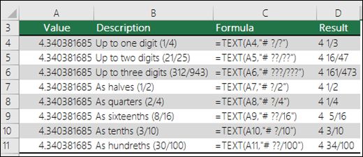
=TEXT(4.34 ,«# ?/?») |
Fraction, like 4 1/3 |
|
=TRIM(TEXT(0.34,«# ?/?»)) |
Fraction, like 1/3. Note this uses the TRIM function to remove the leading space with a decimal value. |
|
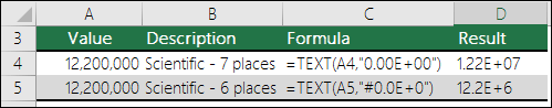
=TEXT(12200000,«0.00E+00») |
Scientific notation, like 1.22E+07 |
|
=TEXT(1234567898,«[<=9999999]###-####;(###) ###-####») |
Special (Phone number), like (123) 456-7898 |
|
=TEXT(1234,«0000000») |
Add leading zeros (0), like 0001234 |
|
=TEXT(123456,«##0° 00′ 00»») |
Custom — Latitude/Longitude |
Note: Although you can use the TEXT function to change formatting, it’s not the only way. You can change the format without a formula by pressing CTRL+1 (or  +1 on the Mac), then pick the format you want from the Format Cells > Number dialog.
Download our examples
You can download an example workbook with all of the TEXT function examples you’ll find in this article, plus some extras. You can follow along, or create your own TEXT function format codes.
Download Excel TEXT function examples
Other format codes that are available
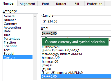
You can use the Format Cells dialog to find the other available format codes:
-
Press Ctrl+1 (
 +1 on the Mac) to bring up the Format Cells dialog.
 -
Select the format you want from the Number tab.
-
Select the Custom option,
-
The format code you want is now shown in the Type box. In this case, select everything from the Type box except the semicolon (;) and @ symbol. In the example below, we selected and copied just mm/dd/yy.
-
Press Ctrl+C to copy the format code, then press Cancel to dismiss the Format Cells dialog.
-
Now, all you need to do is press Ctrl+V to paste the format code into your TEXT formula, like: =TEXT(B2,»mm/dd/yy«). Make sure that you paste the format code within quotes («format code»), otherwise Excel will throw an error message.

Format codes by category
Following are some examples of how you can apply different number formats to your values by using the Format Cells dialog, then use the Custom option to copy those format codes to your TEXT function.
Why does Excel delete my leading 0’s?
Excel is trained to look for numbers being entered in cells, not numbers that look like text, like part numbers or SKU’s. To retain leading zeros, format the input range as Text before you paste or enter values. Select the column, or range where you’ll be putting the values, then use CTRL+1 to bring up the Format > Cells dialog and on the Number tab select Text. Now Excel will keep your leading 0’s.
If you’ve already entered data and Excel has removed your leading 0’s, you can use the TEXT function to add them back. You can reference the top cell with the values and use =TEXT(value,»00000″), where the number of 0’s in the formula represents the total number of characters you want, then copy and paste to the rest of your range.
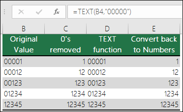
If for some reason you need to convert text values back to numbers you can multiply by 1, like =D4*1, or use the double-unary operator (—), like =—D4.
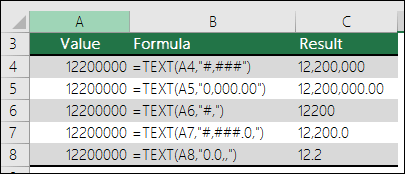
Excel separates thousands by commas if the format contains a comma (,) that is enclosed by number signs (#) or by zeros. For example, if the format string is «#,###», Excel displays the number 12200000 as 12,200,000.
A comma that follows a digit placeholder scales the number by 1,000. For example, if the format string is «#,###.0,», Excel displays the number 12200000 as 12,200.0.
Notes:
-
The thousands separator is dependent on your regional settings. In the US it’s a comma, but in other locales it might be a period (.).
-
The thousands separator is available for the number, currency and accounting formats.
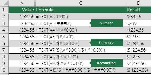
Following are examples of standard number (thousands separator and decimals only), currency and accounting formats. Currency format allows you to insert the currency symbol of your choice and aligns it next to your value, while accounting format will align the currency symbol to the left of the cell and the value to the right. Note the difference between the currency and accounting format codes below, where accounting uses an asterisk (*) to create separation between the symbol and the value.
To find the format code for a currency symbol, first press Ctrl+1 (or +1 on the Mac), select the format you want, then choose a symbol from the Symbol drop-down:
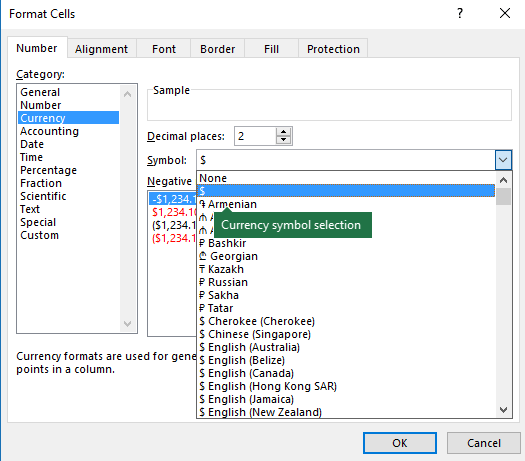
Then click Custom on the left from the Category section, and copy the format code, including the currency symbol.
Note: The TEXT function does not support color formatting, so if you copy a number format code from the Format Cells dialog that includes a color, like this: $#,##0.00_);[Red]($#,##0.00), the TEXT function will accept the format code, but it won’t display the color.
You can alter the way a date displays by using a mix of «M» for month, «D» for days, and «Y» for years.
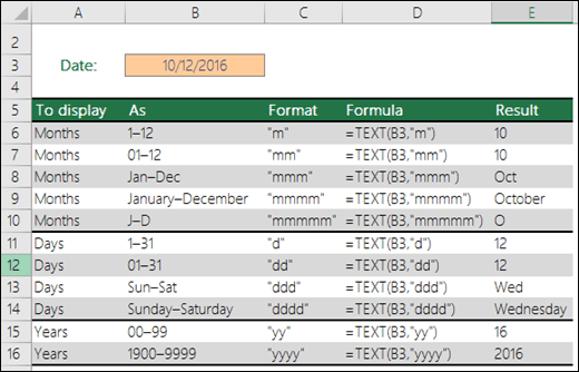
Format codes in the TEXT function aren’t case sensitive, so you can use either «M» or «m», «D» or «d», «Y» or «y».
You can alter the way time displays by using a mix of «H» for hours, «M» for minutes, or «S» for seconds, and «AM/PM» for a 12-hour clock.
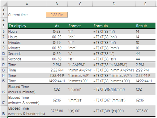
If you leave out the «AM/PM» or «A/P», then time will display based on a 24-hour clock.
Format codes in the TEXT function aren’t case sensitive, so you can use either «H» or «h», «M» or «m», «S» or «s», «AM/PM» or «am/pm».
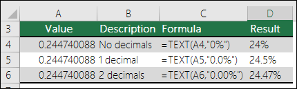
You can alter the way decimal values display with percentage (%) formats.
You can alter the way decimal values display with fraction (?/?) formats.
Scientific notation is a way of displaying numbers in terms of a decimal between 1 and 10, multiplied by a power of 10. It is often used to shorten the way that large numbers display.
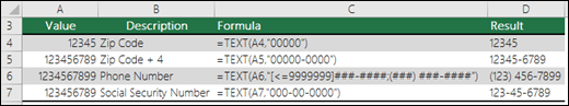
Excel provides 4 special formats:
-
Zip Code — «00000»
-
Zip Code + 4 — «00000-0000»
-
Phone Number — «[<=9999999]###-####;(###) ###-####»
-
Social Security Number — «000-00-0000»
Special formats will be different depending on locale, but if there aren’t any special formats for your locale, or if these don’t meet your needs then you can create your own through the Format Cells > Custom dialog.
Common scenario
The TEXT function is rarely used by itself, and is most often used in conjunction with something else. Let’s say you want to combine text and a number value, like “Report Printed on: 03/14/12”, or “Weekly Revenue: $66,348.72”. You could type that into Excel manually, but that defeats the purpose of having Excel do it for you. Unfortunately, when you combine text and formatted numbers, like dates, times, currency, etc., Excel doesn’t know how you want to display them, so it drops the number formatting. This is where the TEXT function is invaluable, because it allows you to force Excel to format the values the way you want by using a format code, like «MM/DD/YY» for date format.
In the following example, you’ll see what happens if you try to join text and a number without using the TEXT function. In this case, we’re using the ampersand (&) to concatenate a text string, a space (» «), and a value with =A2&» «&B2.
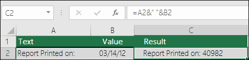
As you can see, Excel removed the formatting from the date in cell B2. In the next example, you’ll see how the TEXT function lets you apply the format you want.
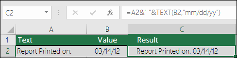
Our updated formula is:
-
Cell C2:=A2&» «&TEXT(B2,»mm/dd/yy») — Date format
Frequently Asked Questions
Yes, you can use the UPPER, LOWER and PROPER functions. For example, =UPPER(«hello») would return «HELLO».
Yes, but it takes a few steps. First, select the cell or cells where you want this to happen and use Ctrl+1 to bring up the Format > Cells dialog, then Alignment > Text control > check the Wrap Text option. Next, adjust your completed TEXT function to include the ASCII function CHAR(10) where you want the line break. You might need to adjust your column width depending on how the final result aligns.
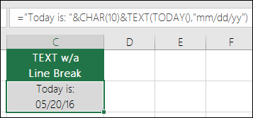
In this case, we used: =»Today is: «&CHAR(10)&TEXT(TODAY(),»mm/dd/yy»)
This is called Scientific Notation, and Excel will automatically convert numbers longer than 12 digits if a cell(s) is formatted as General, and 15 digits if a cell(s) is formatted as a Number. If you need to enter long numeric strings, but don’t want them converted, then format the cells in question as Text before you input or paste your values into Excel.
See Also
Create or delete a custom number format
Convert numbers stored as text to numbers
All Excel functions (by category)
See all How-To Articles
In this tutorial, you will learn how to convert a spreadsheet to a delimited text file from Excel or Google Sheets.
Convert Spreadsheet to Delimited TXT
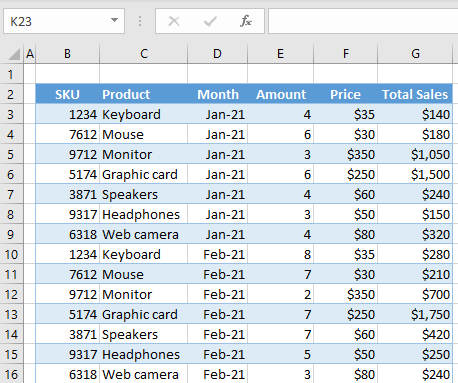
To convert a spreadsheet to a text file, first open it in Excel. The following example will show how to save the table below as text without losing the column separators.
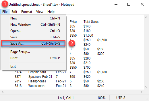
1. To save as a text file, from the Ribbon, go to File > Save As.
2. Choose document type Text (Tab delimited (*.txt).
3. Then press Save.
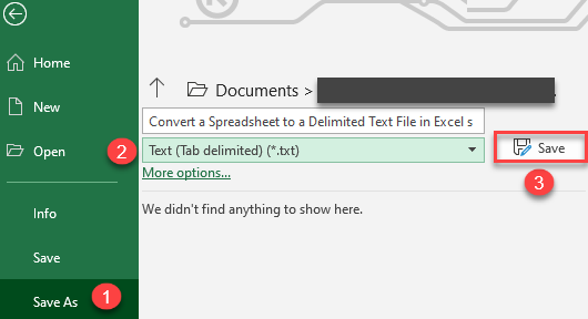
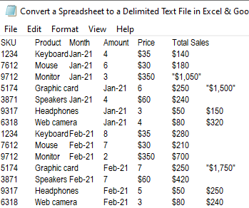
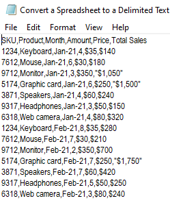
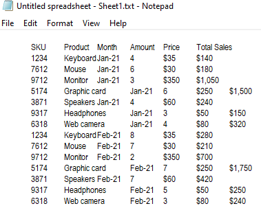
As a result, a text (tab-delimited) file is saved in the location you specified with all columns separated by a tabulator. When you open the file in a text editor (such as Notepad), it looks like the picture below.
Convert an Excel File to a Comma-Delimited CSV File
You can also convert a spreadsheet to a comma-delimited text file in a similar way.
1. In the Ribbon, go to File > Save As.
2. Choose document type CSV (Comma delimited (*.csv).
3. Then press Save.
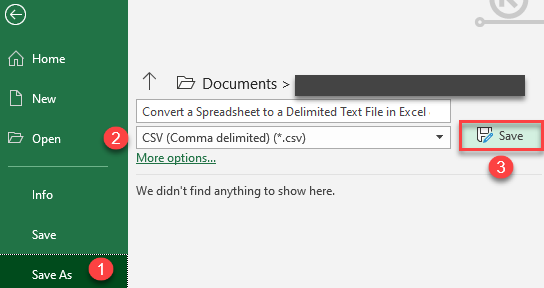
Now, all columns in the CSV file are separated by a comma. When you open the file in a text editor (such as Notepad), it looks like the picture below.
Note: From the text editor, the CSV file can be saved as a text (.txt) file if necessary.
Convert a Google Sheets File to a Delimited TXT File
There are two steps to convert a Google Sheets spreadsheet to a tab delimited file:
- Save a sheet as a Tab-separated values (.tsv) file.
- Save that file as a tab delimited (.txt) file.
In the Menu, go to File > Download > Tab-separated values (.tsv, current sheet).
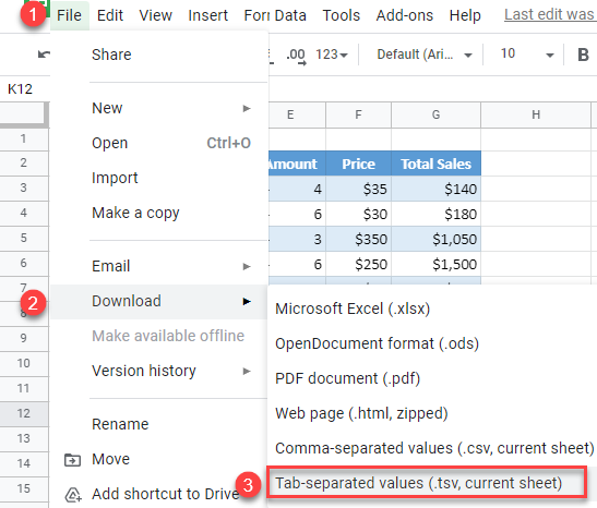
As a result, you get a TSV file that save as a text file. Open the TSV file in a text editor (such as Notepad) and save it with the .txt file extension.
1. To do this, go to File > Save As (or use the keyboard shortcut F12).
2. In the pop-up window, (1) set the document type to Text Documents (*.txt), and (2) click Save.
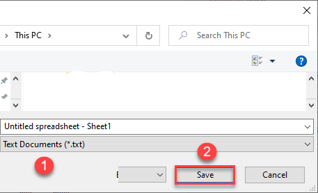
The final output is the text file with the tabular delimiter.
Convert a Google Sheets File to a Comma-Delimited (.csv) File
To convert a Google Sheets file to a comma-delimited file, go to File > Download > Comma-separated values (.csv, current sheet).
How to convert an Excel column into a comma separated list?
- Open your excel sheet and select the cells of the column that you want to process.
- Now open word document, right click on it and from the context menu, select ‘Paste Options’ as ‘Keep texts only’.
- Now press ‘CTRL + H’ to open the ‘Find and Replace’ dialog.
How do I add a comma to a list in Excel?
Select a blank cell such as cell B1 which is adjacent to the cell you want to add comma at end, enter the formula =A1&”,”, and then press the Enter key.
How do I add a comma in front of a number in Excel?
How to add comma before number in Excel?
- Firstly, you need to identify the location of the number.
- Go to C1, and type this formula =REPLACE(A1,B1,1,”,”&MID(A1,B1,1)), and press Enter key, and then drag autofill handle down to apply this formula to cells.
- After free installing Kutools for Excel, please do as below:
How do I change the comma in Excel?
Remove comma from Text String
- Select the dataset.
- Click the Home tab.
- In the Editing group, click on the Find & Replace option.
- Click on Replace. This will open the Find and Replace dialog box.
- In the ‘Find what:’ field, enter , (a comma)
- Leave the ‘Replace with:’ field empty.
- Click on Replace All button.
Where is the comma in Excel?
Explanation: to find the position of the comma, use the FIND function (position 6). =LEFT(A2,FIND(“,”, A2)-1) reduces to =LEFT(A2,6-1). =LEFT(A2,5) extracts the 5 leftmost characters and gives the desired result (Smith). 3.
Why won’t Excel let me insert a page break?
If manual page breaks that you add don’t work, you may have the Fit To scaling option selected (Page Layout tab -> Page Setup group -> click Dialog Box Launcher Button image -> Page). Change the scaling to Adjust to instead. On the picture below, you can see 3 horizontal page breaks added.
What is a page break in Excel?
Insert a page break in Excel to specify where a new page will begin in the printed copy.
How do you create a page in Excel?
Right-click the selected cell and then select “Insert Page Break.” Alternatively, click the “Page Layout” tab, the “Breaks” drop-down button in the Page Setup group and then select “Insert Page Break.” Your new page break is marked by the solid blue line.
How do I split my screen vertically in Excel?
Vertically Split Screen Select the column which you want to split to appear on the left of and select (Window > Split). To adjust the split panes you can drag them to the desired position. You can also use the mouse to drag and resize the panes.
How do I convert Excel columns to comma separated text?
How to convert an Excel column into a comma separated list?
- Open your excel sheet and select the cells of the column that you want to process.
- Now open word document, right click on it and from the context menu, select ‘Paste Options’ as ‘Keep texts only’.
- Now press ‘CTRL + H’ to open the ‘Find and Replace’ dialog.
How can I get column values as comma separated in SQL?
In SQL Server, we can make a comma separated list by using COALESCE as shown in below. Suppose we have following data in Employee table and we need to make a semicolon separated list of EmailIDs to send mail, then we can use COALESCE as shown in below fig.
How do I put multiple cells into one comma separated?
Combine data using the CONCAT function
- Select the cell where you want to put the combined data.
- Type =CONCAT(.
- Select the cell you want to combine first. Use commas to separate the cells you are combining and use quotation marks to add spaces, commas, or other text.
- Close the formula with a parenthesis and press Enter.
How do you convert columns to comma Separated?
1. Select a blank cell adjacent to the list’s first data, for instance, the cell C1, and type this formula =CONCATENATE(TRANSPOSE(A1:A7)&”,”) (A1:A7 is the column you will convert to comma serrated list, “,” indicates the separator you want to separate the list). See screenshot below: 2.
How do I get comma separated values in multiple rows in SQL?
Code follows
- create FUNCTION [dbo].[fn_split](
- @delimited NVARCHAR(MAX),
- @delimiter NVARCHAR(100)
- ) RETURNS @table TABLE (id INT IDENTITY(1,1), [value] NVARCHAR(MAX))
- AS.
- BEGIN.
- DECLARE @xml XML.
- SET @xml = N” + REPLACE(@delimited,@delimiter,”) + ”
What is the shortcut to merge cells in Excel?
Shortcut is “ALT + H + M + A”. Merge Cells: This will only merge the selected cells into one. Shortcut is “ALT + H + M + M”.
How to convert a column to a comma separated list in Excel?
Use this tool to convert a column into a Comma Separated List Copy your column of text in Excel Paste the column here (into the leftmost textbox) Copy your comma separated list from the rightmost textbox
How to input a comma separated string in Python?
1 Input a comma – separated string using raw_input () method. 2 Split the elements delimited by comma (,) and assign it to the list, to split string, use string.split () method. 3 The converted list will contains string elements. 4 Convert elements to exact integers: Traverse each number in the list by using for…in loop. 5 Print the list.
How to convert a column to a list in Excel?
If you want to convert a column list of data to a list separated by comma or other separators, and output the result into a cell as shown as below, you can get it done by CONCATENATE function or running a VBA in Excel. Convert column list to comma separated list with CONCATENATE function.
How to convert a list to a comma serrated list?
Select a blank cell adjacent to the list’s first data, for instance, the cell C1, and type this formula =CONCATENATE (TRANSPOSE (A1:A7)&”,”) (A1:A7 is the column you will convert to comma serrated list, “,” indicates the separator you want to separate the list).
How do I convert Excel columns to comma-separated text?
How to convert an Excel column into a comma separated list?
- Open your excel sheet and select the cells of the column that you want to process.
- Now open word document, right click on it and from the context menu, select ‘Paste Options’ as ‘Keep texts only’.
- Now press ‘CTRL + H’ to open the ‘Find and Replace’ dialog.
How do you create a comma-separated string from an ArrayList?
To convert ArrayList to comma-separated String, these are the approaches available in Java.
- Using append() method of StringBuilder.
- Using toString() method.
- Using Apache Commons StringUtils class.
- Using Stream API.
- Using join() method of String class.
How do you convert a list to a comma-separated string in python?
Call str. join(iterable) with a comma, “,” , as str and a list as iterable . This joins each list element into a comma-separated string. If the list contains non-string elements, use str(object) to convert each element to a string first.
How do you add comma-separated values in a string in Java 8?
In Java 8
- List cities = Arrays. asList(“Milan”, “London”, “New York”, “San Francisco”); String citiesCommaSeparated = String.
- String citiesCommaSeparated = cities. stream() . collect(Collectors. joining(“,”)); System.
- String citiesCommaSeparated = cities. stream() . map(String::toUpperCase) . collect(Collectors.
How do you convert columns to comma Separated?
1. Select a blank cell adjacent to the list’s first data, for instance, the cell C1, and type this formula =CONCATENATE(TRANSPOSE(A1:A7)&”,”) (A1:A7 is the column you will convert to comma serrated list, “,” indicates the separator you want to separate the list). See screenshot below: 2.
How do I put multiple cells into one comma separated?
Combine data using the CONCAT function
- Select the cell where you want to put the combined data.
- Type =CONCAT(.
- Select the cell you want to combine first. Use commas to separate the cells you are combining and use quotation marks to add spaces, commas, or other text.
- Close the formula with a parenthesis and press Enter.
How do you convert a String to a separated list?
Approach: This can be achieved with the help of join() method of String as follows.
- Get the List of String.
- Form a comma separated String from the List of String using join() method by passing comma ‘, ‘ and the list as parameters.
- Print the String.
How do you read a comma separated value from a String in Java?
In order to parse a comma-delimited String, you can just provide a “,” as a delimiter and it will return an array of String containing individual values. The split() function internally uses Java’s regular expression API (java. util. regex) to do its job.
How to convert a list to a comma separated string in Java?
Given a List of String, the task is to convert the List to a comma separated String in Java. Approach: This can be achieved with the help of join () method of String as follows. Get the List of String. Form a comma separated String from the List of String using join () method by passing comma ‘, ‘ and the list as parameters. Print the String.
How to convert list of strings to string?
That depends on what you mean by “best”. The least memory intensive is to first calculate the size of the final string, then create a StringBuilder with that capacity and add the strings to it. The StringBuilder will create a string buffer with the correct size, and that buffer is what you get from the ToString method as a string.
How to convert a list to a string in Java 8?
Join the DZone community and get the full member experience. Converting a List to a String with all the values of the List comma separated in Java 8 is really straightforward. Let’s have a look how to do that.
How to remove the last comma in CSV string?
//Remove last comma csv=csv.substring(0, csv.length() -SEPARATOR.length()); System.out.println(csv); //OUTPUT: Milan,London,New York,San Francisco As you can see it’s much more verbose and easier to make mistakes like forgetting to remove the last comma.
When data is imported into Excel it can be in many formats depending on the source application that has provided it.
For example, it could contain names and addresses of customers or employees, but this all ends up as a continuous text string in one column of the worksheet, instead of being separated out into individual columns e.g. name, street, city.
You can split the data by using a common delimiter character. A delimiter character is usually a comma, tab, space, or semi-colon. This character separates each chunk of data within the text string.
A big advantage of using a delimiter character is that it does not rely on fixed widths within the text. The delimiter indicates exactly where to split the text.
You may need to split the data because you may want to sort the data using a certain part of the address or to be able to filter on a particular component. If the data is used in a pivot table, you may need to have the name and address as different fields within it.
This article shows you eight ways to split the text into the component parts required by using a delimiter character to indicate the split points.
Sample Data
The above sample data will be used in all the following examples. Download the example file to get the sample data plus the various solutions for extracting data based on delimiters.
Excel Functions to Split Text
There are several Excel functions that can be used to split and manipulate text within a cell.
LEFT Function
The LEFT function returns the number of characters from the left of the text.
Syntax
= LEFT ( Text, [Number] )- Text – This is the text string that you wish to extract from. It can also be a valid cell reference within a workbook.
- Number [Optional] – This is the number of characters that you wish to extract from the text string. The value must be greater than or equal to zero. If the value is greater than the length of the text string, then all characters will be returned. If the value is omitted, then the value is assumed to be one.
RIGHT Function
The RIGHT function returns the number of characters from the right of the text.
Syntax
= RIGHT ( Text, [Number] )The parameters work in the same way as for the LEFT function described above.
FIND Function
The FIND function returns the position of specified text within a text string. This can be used for locating a delimiter character. Note that the search is case-sensitive.
Syntax
= FIND (SubText, Text, [Start])- SubText – This is a text string that you want to search for.
- Text – This is the text string which is to be searched.
- Start [Optional] – The starting position for the search.
LEN Function
The LEN function will give the length by number of characters of a text string.
Syntax
= LEN ( Text )- Text – This is the text string of which you want to determine the character count.
Extracting Data with the LEFT, RIGHT, FIND and LEN Functions
Using the first row (B3) of the sample data, these functions can be combined to split a text string into sections using a delimiter character.
= FIND ( ",", B3 )You use the FIND function to get the position of the first delimiter character. This will return the value 18.
= LEFT ( B3, FIND( ",", B3 ) - 1 )You can then use the LEFT function to extract the first component of the text string.
Note that FIND gets the position of the first delimiter, but you need to subtract 1 from it so as to not include the delimiter character.
This will return Tabbie O’Hallagan.
= RIGHT ( B3, LEN ( B3 ) - FIND ( ",", B3 ) )It is more complicated to get the next components of the text string. You need to remove the first component from the text by using the above formula.
This formula takes the length of the original text, finds the first delimiter position, which then calculates how many characters are left in the text string after that delimiter.
The RIGHT function then truncates off all the characters up to and including that first delimiter so that the text string gets shorter and shorter as each delimiter character is found.
This will return 056 Dennis Park, Greda, Croatia, 44273
You can now use FIND to locate the next delimiter and the LEFT function to extract the next component, using the same methodology as above.
Repeat for all delimiters, and this will split the text string into component parts.
FILTERXML Function as a Dynamic Array
If you’re using Excel for Microsoft 365, then you can use the FILTERXML function to split text with output as a dynamic array.
You can split a text string by turning it into an XML string by changing the delimiter characters to XML tags. This way you can use the FILTERXML function to extract data.
XML tags are user defined, but in this example, s will represent a sub-node and t will represent the main node.
= "<t><s>" & SUBSTITUTE ( B2, ",", "</s><s>" ) & "</s></t>"Use the above formula to insert the XML tags into your text string.
<t><s>Name</s><s>Street</s><s>City</s><s>Country</s><s>Post Code</s></t>This will return the above formula in the example.
Note that each of the nodes defined is followed by a closing node with a backslash. These XML tags define the start and finish of each section of the text, and effectively act in the same way as delimiters.
=TRANSPOSE(
    FILTERXML(
        "<t><s>" &
        SUBSTITUTE(
            B3,
            ",",
            "</s><s>"
        ) & "</s></t>",
        "//s"
    )
)
The above formula will insert the XML tags into the original string and then use these to split out the items into an array.
As seen above, the array will spill each item into a separate cell. Using the TRANSPOSE function causes the array to spill horizontally instead of vertically.
FILTERXML Function to Split Text
If your version of Excel doesn’t have dynamic arrays, then you can still use the FILTERXML function to extract individual items.
= FILTERXML (
    "<t><s>" &
    SUBSTITUTE (
        B3,
        ",",
        "</s><s>"
    ) & "</s></t>",
    "//s"
)
You can now break the string into sections using the above FILTERXML formula.
This will return the first section Tabbie O’Hallagan.
= FILTERXML (
    "<t><s>" &
    SUBSTITUTE (
        B3,
        ",",
        "</s><s>"
    ) & "</s></t>",
    "//s[2]"
)
To return the next section, use the above formula.
This will return the second section of the text string 056 Dennis Park.
You can use this same pattern to return any part of the sample text, just change the [2] found in the formula accordingly.
Flash Fill to Split Text
Flash Fill allows you to put in an example of how you want your data split.
You can check out this guide on using flash fill to clean your data for more details.
You then select the first cell of where you want your data to split and click on Flash Fill. Excel will populate the remaining rows from your example.
Using the sample data, enter Name into cell C2, then Tabbie O’Hallagan into cell C3.
Flash fill should automatically fill in the remaining data names from the sample data. If it doesn’t, you can select cell C4, and click on the Flash Fill icon in the Data Tools group of the Data tab of the Excel ribbon.
Similarly, you can add Street into cell D2, City into cell E2, Country into cell F2, and Post Code into cell G2.
Select the subsequent cells (D2 to G2) individually, and click on the Flash Fill icon. The rest of the text components will be populated into these columns.
Text to Columns Command to Split Text
This Excel functionality can be used to split text in a cell into sections based on a delimiter character.
- Select the entire sample data range (B2:B12).
- Click on the Data tab in the Excel ribbon.
- Click on the Text to Columns icon in the Data Tools group of the Excel ribbon and a wizard will appear to help you set up how the text will be split.
- Select Delimited on the option buttons.
- Press the Next button.
- Select Comma as the delimiter, and uncheck any other delimiters.
- Press the Next button.
- The Data Preview window will display how your data will be split. Choose a location to place the output.
- Click on Finish button.
Your data will now be displayed in columns on your worksheet.
Convert the Data into a CSV File
This will only work with commas as delimiters, since a CSV (comma separated value) file depends on commas to separate the values.
Open Notepad and copy and paste the sample data into it. You can open Notepad by typing Notepad into the search box at the left of the Windows task bar or locate it in the application list.
Once you have copied the data into Notepad, save it off by using File ➜ Save As from the menu. Enter a filename with a .csv suffix e.g. Split Data.csv.
You can then open this file in Excel. Select the csv file in the browser file type drop down and click OK. Your data will automatically appear with each component in separate columns.
VBA to Split Text
VBA is the programming language that sits behind Excel and allows you to write your own code to manipulate data, or to even create your own functions.
To access the Visual Basic Editor (VBE), you use Alt + F11.
Sub SplitText()

Dim MyArray() As String, Count As Long, i As Variant

For n = 2 To 12
	MyArray = Split(Cells(n, 2), ",")
	Count = 3
	For Each i In MyArray
		Cells(n, Count) = i
		Count = Count + 1
	Next i
Next n

End Sub
Click on Insert in the menu bar, and click on Module. A new pane will appear for the module. Paste in the above code.
This code creates a single dimensional array called MyArray. It then iterates through the sample data (rows 2 to 12) and uses the VBA Split function to populate MyArray.
The split function uses a comma delimiter, so that each section of the text becomes an element of the array.
A counter variable is set to 3 which represents column C, which will be the first column for the split data to be displayed.
The code then iterates through each element in the array and populates each cell with the element. Cell references are based on n for the row, and Count for the column.
The variable Count is incremented in each loop so that the data fills across the row, and then downwards.
Power Query to Split Text
Power Query in Excel allows a column to be manipulated into sections using a delimiter character.
Related posts:
- Introduction to power query
- Power query tips and tricks
- Introduction to power query M code
The first thing to do is to define your data source, which is the sample data that you entered into you Excel worksheet.
Click on the Data tab in the Excel ribbon, and then click on Get Data in the Get & Transform Data group of the ribbon.
Click on From File in the first drop down, and then click on From Workbook in the second drop down.
This will display a file browser. Locate your sample data file (the file that you have open) and click on OK.
A navigation pop-up will be displayed showing all the worksheets within your workbook. Click on the worksheet which has the sample data and this will show a preview of the data.
Expand the tree of data in the left-hand pane to show the preview of the existing data.
Click on Transform Data and this will display the Power Query Editor.
Make sure that the single column with the data in it is highlighted. Click on the Split Column icon in the Transform group of the ribbon. Click on By Delimiter in the drop down that appears.
This will display a pop-up window which allows you to select your delimiter. The default is a comma.
Click OK and the data will be transformed into separate columns.
Click on Close and Load in the Close group of the ribbon, and a new worksheet will be added to your workbook with a table of the data in the new format.
Power Pivot Calculated Column to Split Text
You can use Power Pivot to split the text by using calculated columns.
Click on the Power Pivot tab in the Excel ribbon and then click on the Add to Data Model icon in the Tables group.
Your data will be automatically detected and a pop-up will show the location. If this is not the correct location, then it can be re-set here.
Leave the My table has headers check box un-ticked in the pop-up, as we want to split the header as well.
Click on OK and a preview screen will be displayed.
Right-click on the header for your data column (Column1) and click on Insert Column in the pop-up menu. This will insert a calculated column where a formula can be entered.
= LEFT ( [Column1], FIND ( ",", [Column1] ) - 1 )In the formula bar, insert the above formula.
This works in a similar way to the functions described in method 1 of this article.
This formula will provide the Name component within the text string.
Insert another calculated column using the same methodology as the first calculated column.
= LEFT (
    RIGHT ( [Column1], LEN ( [column1] ) - LEN ( [Calculated Column 1] ) - 1 ),
    FIND (
        ",",
        RIGHT ( [Column1], LEN ( [column1] ) - LEN ( [Calculated Column 1] ) - 1 )
    ) - 1
)
Insert the above formula into the formula bar.
This is a complicated formula, and you may wish to break it into sections using several calculated columns.
This will provide the Street component in the text string.
You can continue modifying the formula to create calculated columns for all the other components of the text string.
The problem with a pivot table is that it needs a numeric value as well as text values. As the sample data is text only, a numeric value needs to be added.
Click on the first cell in the Add Column column and enter the formula =1 in the formula bar.
This will add the value of 1 all the way down that column. Click on the Pivot Table icon in the Home tab of the ribbon.
Click on Pivot Table in the pop-up menu. Specify the location of your pivot table in the first pop-up window and click OK. If the Pivot Table Fields pane does not automatically display, right click on the pivot table skeleton and select Show Field List.
Click on the Calculated Columns in the Field List and place these in the Rows window.
our pivot table will now show the individual components of the text string.
Conclusions
Dealing with comma or other delimiter separated data can be a big pain if you don’t know how to extract each item into its own cell.
Thankfully, Excel has quite a few options that will help with this common task.
Which one do you prefer to use?
About the Author
John is a Microsoft MVP and qualified actuary with over 15 years of experience. He has worked in a variety of industries, including insurance, ad tech, and most recently Power Platform consulting. He is a keen problem solver and has a passion for using technology to make businesses more efficient.
So earlier we had CONCAT, and CONCATENATE function to concatenate multiple cells. But if we wanted to supply a range for joining cells with a delimiter (say a comma) then it is really tricky with these functions. But now Excel has introduced a new function called TEXTJOIN Function that can be used to concatenate ranges with a lot more flexibility.
In this article, we will learn how to concatenate cell values of a range with comma using TEXTJOIN function. For users who don’t have this function we will discuss other methods of concatenating range values with comma.
Generic Formula
=TEXTJOIN(«,»,TRUE,text_range1,[text_range2]…)
Comma («,») : This is the delimiter we want to use. Since in this article we are concentrating on concatenating cells with commas.
TRUE : For ignoring blank cells in the range.
Text_range1 : This is the range whose cells have values you want to concatenate.
[Text_range2] : The other ranges if you want to join in the text with commas.
Let’s see an example to make things clear.
Example: Join Cell Values of Ranges With Comma as Delimiter
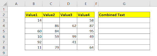
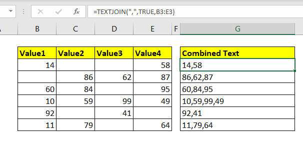
Here, we have some values in range B2:E8. We need to join the texts of each cell in a row.
Let’s implement the formula we have and drag it down.
You can see that we have a string which is a result of concatenation of texts with commas.
Let’s say if you want to concatenate the range B3:E3 and B7:E7. So the formula will be:
It will concatenate all the texts ignoring the blank cells.
How does it work?
The formula is simple. The TEXTJOIN function requires the delimiter with which you want to join text with. The second variable is set to be true so that it ignores the blank cells.
Now if any cell has invisible values like space then you will see an extra comma in between the joined text.
To avoid spaces, use the TRIM function to strip them out.
Concatenating Cells with Commas in Excel 2016 and Older
The problem is that the TEXTJOIN function is only available to Excel 2019 and 365. So if you want to concatenate the cells with commas, we’ll need to use a trick.
So to concatenate cells in a row with commas do this.
In a cell, write «=» to start the formula and select the range as shown below.

Now press F2 and select the range in the formula bar or cell.

Press F9 key.

Now remove the equals and curly braces. You have the cells joined with commas.

But this way is not that effective for too many operations.
So do we have any other way to combine texts with a given delimiter in Excel? The other way is the VBA way. Let’s create one UDF to do this.
Function JoinText(delimiter As String, rng As Range)

Dim res As String

For Each cell In rng

 If Trim(cell.Value) <> "" Then

  res = res & Trim(cell.Value) & delimiter

 End If

Next cell
res = Left(res, Len(res) - 1)

JoinText = res

End Function
Press CTRL+F11 to open the VB Editor. Right click on the workbook and insert a module. Copy the code above and paste in the module’s code area.

Now use this formula to join text with any delimiter you want to.

This formula will work in any version of Excel. You can download the workbook below to use this formula immediately.
So yeah guys, this is how you can join text with comma delimiter in Excel. I hope it was helpful for you. If you have any questions regarding this topic or any other excel related topic, ask in the comments section below. Till then keep Excelling.
Related Articles:
Split Numbers and Text from String in Excel 2016 and Older: When we didn’t have TEXTJOIN function we used LEFT and RIGHT functions with some other functions to split numeric and nonnumeric characters from a string.
Extract Text From A String In Excel Using Excel’s LEFT And RIGHT Function: To remove text in excel from string we can use excel’s LEFT and RIGHT function. These functions help us chop strings dynamically.
Remove leading and trailing spaces from text in Excel: Leading and trailing spaces are hard to recognize visually and can mess up your data. Stripping these characters from the string is a basic and most important task in data cleaning. Here’s how you can do it easily in Excel.
Remove Characters From Right: To remove characters from the right of a string in Excel, we use the LEFT function. Yes, the LEFT function. The LEFT function retains the given number of characters from LEFT and removes everything from its right.
Remove unwanted characters in Excel: To remove unwanted characters from a string in Excel, we use the SUBSTITUTE function. The SUBSTITUTE function replaces the given characters with another given character and produces a new altered string.
How to Remove Text in Excel Starting From a Position in Excel: To remove text from a starting position in a string, we use the REPLACE function of Excel. This function help us determine the starting position and number of characters to strip.
Popular Articles:
50 Excel Shortcuts to Increase Your Productivity | Get faster at your task. These 50 shortcuts will make you work even faster on Excel.
How to use Excel VLOOKUP Function| This is one of the most used and popular functions of excel that is used to lookup value from different ranges and sheets.
How to use the Excel COUNTIF Function| Count values with conditions using this amazing function. You don’t need to filter your data to count specific values. Countif function is essential to prepare your dashboard.
How to Use SUMIF Function in Excel | This is another dashboard essential function. This helps you sum up values on specific conditions.