Excel this row in formula

Функция СТРОКА в Excel используется когда вы хотите получить значение номера строки в которой находится конкретная ячейка.

Что возвращает функция

Функция возвращает порядковый номер строки в которой находится нужная ячейка с данными. Например, =ROW(B4) или =СТРОКА(B4) вернет “4”, так как ячейка «B4: находится в четвертой строке таблицы.

Синтаксис

=ROW([reference]) — английская версия

=СТРОКА([ссылка]) — русская версия

Аргументы функции

• [reference] ([ссылка]) — необязательный аргумент, который ссылается на ячейку или диапазон ячеек. Если при использовании функции СТРОКА(ROW) аргумент не указан, то функция отображает номер строки для той ячейки, в которой находится функция СТРОКА(ROW).

Дополнительная информация

• Если аргумент функции ссылается на диапазон ячеек, то функция вернет минимальное значение из указанного диапазона. Например, =ROW(B5:D10) или =СТРОКА(B5:D10), функция СТРОКА вернет значение «5»;
• Если аргумент функции ссылается на массив, функция вернет номера строк в которых находится каждый элемент указанного массива;
• Аргумент функции не может ссылаться на несколько ссылок или адресов;

Примеры использования функции ROW (СТРОКА) в Excel

Пример 1. Вычисляем номер строки ячейки

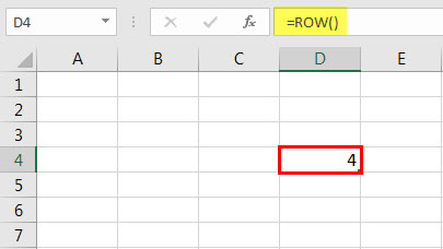
Если вы введете =СТРОКА() или =ROW() в любой ячейке => функция вернет номер строки, в которой находится ячейка с этой функцией.

Пример 2. Вычисляем номер строки конкретной ячейки

Если вы укажете ссылку на ячейку с помощью функции СТРОКА или ROW, она вернет номер строки этой ячейки.

The ROW function in Excel is a worksheet function in Excel that is used to show the current index number of the row of the selected or target cell. It is a built-in function and takes only one argument as the reference. The method to use this function is as follows: =ROW( Value ). It will only show the cell’s row number, not its value.

For example, =ROW(A5) returns 5 because A5 is the fifth row in the Excel spreadsheet.

The ROW function in Excel returns the first-row number within a supplied reference or if no reference is supplied. In addition, the ROW function in Excel returns the current row number in the currently active Excel spreadsheet. The ROW function is a built-in Excel function categorized as Lookup and Reference. The ROW function in Excel always returns the positive numeric value.

Row Formula Excel

Below is the ROW formula for Excel.

Reference is the argument accepted by the ROW formula in Excel, which is a cell or range of cells for which we want the row number.

Argument Value	Cell Formula	Explanation
Nothing	3	Returns the ROW number of the cell the formula is types in
A Cell Reference	1	Returnsthe ROW number 1
A Range	2	Returns the Row number 2

In the first case, we have omitted the reference value, so the output will be the cell’s row number in which we typed the row formula in Excel. In the second case, we have provided the cell referenceCell reference in excel is referring the other cells to a cell to use its values or properties. For instance, if we have data in cell A2 and want to use that in cell A1, use =A2 in cell A1, and this will copy the A2 value in A1.read more B1, so the row number of cell B1 is row 1. Suppose the reference is a range of cells inserted as a vertical array (in the third case) that is E2:E10. Then, the ROW function in Excel will return the row number of the topmost rows in the specified range. Hence, the output in the third case will be 2.

The ROW function in Excel accepts one input (reference), which is optional. In addition, whenever there is a square bracket [] in an argument, it denotes that the argument is optional. So, if we do not provide any input, the ROW function in Excel will return the row number of the active cell.

How to Use ROW Function in Excel?

The ROW function in Excel is very simple and easy to use. Let us understand the working of ROW in Excel by some examples.

You can download this ROW Function Excel Template here – ROW Function Excel Template

ROW in Excel Example #1

If we write the ROW formula in Excel, e.g., in the third row in any cell, it will return the number 3, which is the row number.

As shown in the figure above, we have written the ROW function in cells B3, C3, D3, and E3. In all cells, the ROW function in Excel returns row number 3. If we write the ROW formula in Excel anywhere else in another cell, suppose in cell AA10, the ROW function in Excel will return the value 10.

When we give an input (a reference) to the row in Excel, for example, if we offer input D323, it will return the row number 323 as an output because we are referring to D323.

We can use the Excel ROW function in multiple ways.

Let us check out the applications of the ROW function in Excel.

ROW in Excel Example #2

Suppose we want to generate the serial number from 1 to any number from any cell and their adjacent cells downwards. Suppose, starting from cell D4. Then, we want to create serial numbers 1,2,3,4…so on.

We will use the ROW function in Excel. For example, in D4, we will write the ROW function that =ROW(D4).

Now, we will drag the ROW formula in Excel downwards. For example, suppose we drag it till D15. Then, we get all the row numbers starting from row number 4 to 15.

If we want this series to start from 1, we must subtract the row number just above the cell from where we begin the series. So, we will subtract row number 3 from each row number to get the desired output.

ROW in Excel Example #3

Another example of the ROW function in Excel. Suppose we have a list of names in a column. We want to highlight those names in even rows . We want to highlight those names in rows 2,4,6,8,…so on.

We have a list of names in column A, “Name 1,” “Name 2,” and “Name 3″….”Name 21.” You can see below in the image that we used the Excel row and the previous Excel ROW function application example to generate the list of cell names starting from A2 to A21. Now, using the ROW function in Excel, we have to highlight those names in the list that are in even rows. So, we have highlighted names in cells A2, A4, A6, and A8…A20.

We will use conditional formatting in excelConditional formatting is a technique in Excel that allows us to format cells in a worksheet based on certain conditions. It can be found in the styles section of the Home tab.read more to achieve the task in this case. We will use another function, EVEN(number), apart from the Excel ROW function. The ROW function in Excel returns a round up positive number and a round down negative number to the nearest even integer.

So, only to format even rows, we will use the conditional formula =EVEN(ROW())=ROW()

We will select the rows that we want to format.

Click the “Conditional Formatting” dropdown in the “Styles” group and choose “New Rule.”

From the “Select a Rule Type” list, choose “Use a formula to determine which cells to format.”

In the “Format values where this formula is true” field, type:

=EVEN(ROW())=ROW().

Click “Format.”

Specify any of the available formats. For instance, to shade all even rows red, click on the “File” tab, click “Red,” and click “OK” twice.

The result will be:

We can specify the rows also that are even and odd, using EVEN, ODD, ROW, and IF functions.

It works like this: if the even of a row is equal to the row number, then print even. If the odd of a row equals the row number, print odd. So, the ROW formula in Excel goes like this.

=IF(EVEN(ROW(A2))=ROW(),”Even”,IF(ODD(ROW(A2)=ROW()),”Odd”))

ROW in Excel Example #4

There is another method for alternate shading rows. We can use the MOD function along with the ROW function in Excel.

=MOD(ROW(),2)=0

The ROW formula above returns the ROW number. The MOD function returns the remainder of its first argument divided by its second. For cells in even-numbered rows, the MOD function returns 0, and the cells in that row are formatted.

Result:

ROW in Excel Example #5

Shading groups of Rows using the row function in Excel

Another example, we want to shade alternate groups of rows. Let us say if we want to shade four rows, four rows of un-shaded rows, four more shaded rows, and so on. We will use Excel’s ROW, MOD, and INT functionINT or integer function in excel returns the nearest integer of a given number and is used when we have many data sets and each data in a different format.read more to round off the numeric value obtained.

=MOD(INT((ROW()-1)/4)+1,2)

Result:

For different-sized groups, we can customize the ROW formula in Excel accordingly. If we change to 2 rows grouping, the formula would be as follows:

=MOD(INT((ROW()-1)/2)+1,2)

Result:

Similarly, for 3 rows grouping,

=MOD(INT((ROW()-1)/3)+1,2)

Result:

Things to Remember About ROW Function in Excel

• If we take the input reference as a range of cells, the Excel ROW function returns the row number of the topmost rows in the specified range. For example, if =ROW(D4:G9), the Excel ROW function would return 4 as the top row is D4, for which the row number is 4.
• Excel ROW function accepts only one input, so we cannot refer to multiple references or addresses.
• If the reference is entered as an array, the ROW function in Excel returns the row number of all the rows in the array.

Row Function in Excel Video

Recommended Articles

This article is a guide to the ROW Function in Excel. Here, we discuss the ROW formula in Excel and how to use the ROW function, along with Excel examples and downloadable Excel templates. You may also look at these useful functions in Excel: –

• Convert Columns to RowThere are two ways to convert columns to rows: 1) using the Excel Ribbon Method. 2) The Mouse Method.read more
• Highlight Every Row in ExcelIn Excel, we can highlight every other row in one of three ways: using an Excel table, conditional formatting, or custom formatting.read more
• How to use VLOOKUP Excel Function?The VLOOKUP excel function searches for a particular value and returns a corresponding match based on a unique identifier. A unique identifier is uniquely associated with all the records of the database. For instance, employee ID, student roll number, customer contact number, seller email address, etc., are unique identifiers.
  read more
• HLOOKUP in ExcelHlookup is a referencing worksheet function that finds and matches the value from a row rather than a column using a reference. Hlookup stands for horizontal lookup, in which we search for data in rows horizontally.read more