
Excel для Microsoft 365 Excel для Интернета Excel 2021 Excel 2019 Excel 2016 Excel 2013 Еще…Меньше
Переход на разные уровни при больших объемах данных в иерархии сводной таблицы всегда занимал много времени, включая многочисленные операции развертывания, свертывания и фильтрации.
Функция быстрого изучения позволяет детализировать куб OLAP или иерархию сводной таблицы на основе модели данных для анализа сведений о данных на разных уровнях. Быстрый обзор позволяет перейти к нужным данным и действует как фильтр при детализации. Соответствующая кнопка отображается при выборе элемента в поле.
Обычно вы начинаете с детализации до следующего уровня иерархии. Ниже рассказывается, как это сделать.
-
В кубе OLAP или сводной таблице модели данных выберите элемент (например, Стандартные в нашем примере) в поле (например, поле Категория в нашем примере).
Одновременно можно выполнить детализацию только по одному элементу.
-
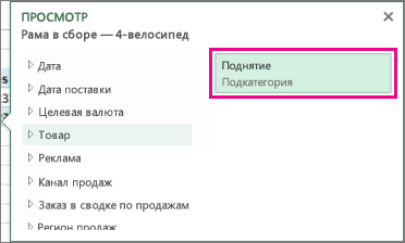
Нажмите кнопку Быстрый обзор
 , которая отображается в правом нижнем углу выделенного фрагмента.
-
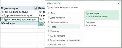
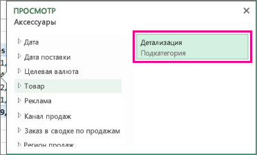
В поле Обзор выберите элемент, который вы хотите изучить, и нажмите кнопку Детализация.
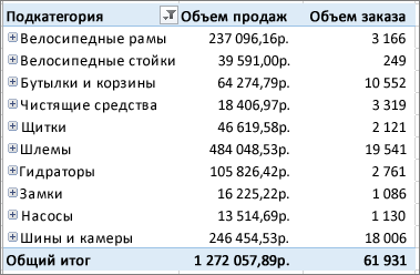
Теперь вы увидите данные подкатегории для этого элемента (в данном случае — вспомогательные продукты).
-
Продолжайте использовать быстрый обзор , пока не хочешь получить нужные данные.
Примечания:
-
Невозможно выполнить детализацию в плоских иерархиях (например, иерархиях, которые отображают атрибуты того же элемента, но не предоставляют данные на следующем уровне) или других иерархиях, в которых нет данных на нескольких уровнях.
-
Если у вас есть сгруппированные элементы в сводной таблице, вы можете детализировать имя группы так же, как и другие элементы.
-
Нельзя детализировать именованные наборы (наборы элементов, которые часто используются или объединяют элементы из разных иерархий).
-
 , которая отображается в правом нижнем углу выделенного фрагмента.
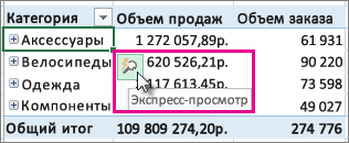
Детализация, чтобы изучить общие сведения о картине
После детализации можно выполнить детализацию для анализа сводных данных. Несмотря на то , что отмена на панели быстрого доступа возвращает вас к месту начала, детализация позволяет создать резервную копию любого другого пути, чтобы получить более подробные аналитические сведения.
-
В иерархии сводной таблицы, которую вы детализировали, выберите элемент, по которому вы хотите детализировать.
-
Нажмите кнопку Быстрый обзор
, которая отображается в правом нижнем углу выделенного фрагмента. -
В поле Обзор выберите элемент, который вы хотите изучить, а затем нажмите кнопку Детализация.
Теперь вы видите данные с более высокого уровня.
-
Продолжайте использовать быстрый обзор , пока не хочешь получить нужные данные.
Примечания:
-
Можно выполнить детализацию нескольких уровней иерархии одновременно. Щелкните правой кнопкой мыши элемент, для которого требуется выполнить детализацию, выберите пункт Детализация и детализация, а затем выберите уровень, до которого требуется выполнить детализацию.
-
Если в сводной таблице есть сгруппированные элементы, можно выполнить детализацию до имени группы.
-
Невозможно выполнить детализацию до именованных наборов (наборы элементов, которые часто используются или объединяют элементы из разных иерархий).
-
Переход на разные уровни при больших объемах данных в иерархии сводной таблицы всегда занимал много времени, включая многочисленные операции развертывания, свертывания и фильтрации.
Функция быстрого изучения позволяет детализировать куб OLAP или иерархию сводной таблицы на основе модели данных для анализа сведений о данных на разных уровнях. Быстрый обзор позволяет перейти к данным, которые вы хотите просмотреть, и действует как фильтр при детализации. Соответствующая кнопка отображается при выборе элемента в поле.
Обычно вы начинаете с детализации до следующего уровня иерархии. Ниже рассказывается, как это сделать.
-
В кубе OLAP или сводной таблице модели данных выберите элемент (например, Стандартные в нашем примере) в поле (например, поле Категория в нашем примере).
Одновременно можно выполнить детализацию только по одному элементу.
-
Нажмите кнопку Быстрый обзор
, которая отображается в правом нижнем углу выделенного фрагмента.
-
В поле Обзор выберите элемент, который вы хотите изучить, и нажмите кнопку Детализация.
Теперь вы увидите данные подкатегории для этого элемента (в данном случае — вспомогательные продукты).
-
Продолжайте использовать быстрый обзор , пока не хочешь получить нужные данные.
Примечания:
-
Невозможно выполнить детализацию в плоских иерархиях (например, иерархиях, которые отображают атрибуты того же элемента, но не предоставляют данные на следующем уровне) или других иерархиях, в которых нет данных на нескольких уровнях.
-
Если у вас есть сгруппированные элементы в сводной таблице, вы можете детализировать имя группы так же, как и другие элементы.
-
Нельзя детализировать именованные наборы (наборы элементов, которые часто используются или объединяют элементы из разных иерархий).
-
Детализация, чтобы изучить общие сведения о картине
После детализации можно выполнить детализацию для анализа сводных данных. Несмотря на то , что отмена на панели быстрого доступа возвращает вас к месту начала, детализация позволяет создать резервную копию любого другого пути, чтобы получить более подробные аналитические сведения.
-
В иерархии сводной таблицы, которую вы детализировали, выберите элемент, по которому вы хотите детализировать.
-
Нажмите кнопку Быстрый обзор
, которая отображается в правом нижнем углу выделенного фрагмента. -
В поле Обзор выберите элемент, который вы хотите изучить, а затем нажмите кнопку Детализация.
Теперь вы видите данные с более высокого уровня.
-
Продолжайте использовать быстрый обзор , пока не хочешь получить нужные данные.
Примечания:
-
Можно выполнить детализацию нескольких уровней иерархии одновременно. Щелкните правой кнопкой мыши элемент, для которого требуется выполнить детализацию, выберите пункт Детализация и детализация, а затем выберите уровень, до которого требуется выполнить детализацию.
-
Если в сводной таблице есть сгруппированные элементы, можно выполнить детализацию до имени группы.
-
Невозможно выполнить детализацию до именованных наборов (наборы элементов, которые часто используются или объединяют элементы из разных иерархий).
-
Если у вас есть классическое приложение Excel, можно использовать кнопку Открыть в Excel , чтобы открыть книгу и детализировать данные сводной таблицы.
Дополнительные сведения
Вы всегда можете задать вопрос специалисту Excel Tech Community или попросить помощи в сообществе Answers community.
См. также
Создание сводной таблицы для анализа внешних данных
Создание сводной таблицы для анализа данных в нескольких таблицах
Упорядочение полей сводной таблицы с помощью списка полей
Группировка и отмена группировки данных в отчете сводной таблицы
Нужна дополнительная помощь?
A hierarchy in Data Model is a list of nested columns in a data table that are considered as a single item when used in a Power PivotTable. For example, if you have the columns − Country, State, City in a data table, a hierarchy can be defined to combine the three columns into one field.
In the Power PivotTable Fields list, the hierarchy appears as one field. So, you can add just one field to the PivotTable, instead of the three fields in the hierarchy. Further, it enables you to move up or down the nested levels in a meaningful way.
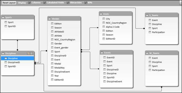
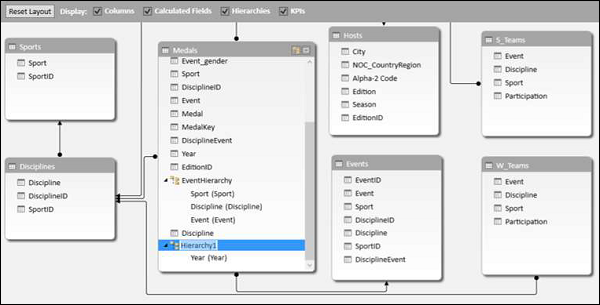
Consider the following Data Model for illustrations in this chapter.
Creating a Hierarchy
You can create Hierarchies in the diagram view of the Data Model. Note that you can create a hierarchy based on a single data table only.
-
Click on the columns − Sport, DisciplineID and Event in the data table Medal in that order. Remember that the order is important to create a meaningful hierarchy.
-
Right-click on the selection.
-
Select Create Hierarchy from the dropdown list.
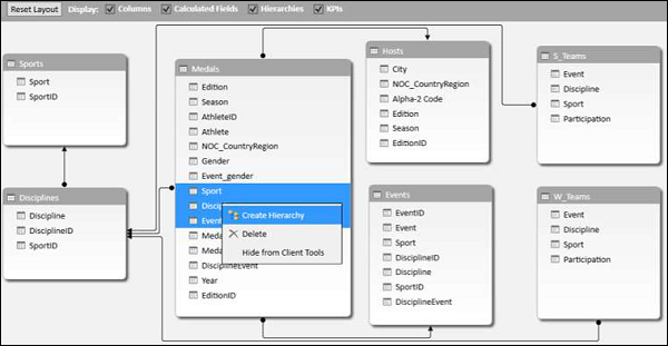
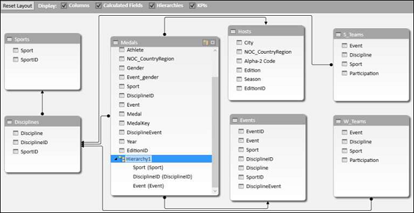
The hierarchy field with the three selected fields as the child levels gets created.
Renaming a Hierarchy
To rename the hierarchy field, do the following −
-
Right click on Hierarchy1.
-
Select Rename from the dropdown list.
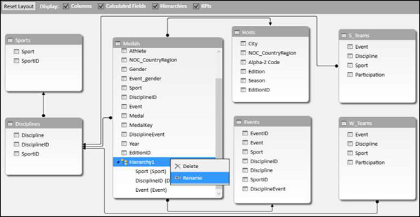
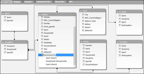
Type EventHierarchy.
Creating a PivotTable with a Hierarchy in Data Model
You can create a Power PivotTable using the hierarchy that you created in the Data Model.
-
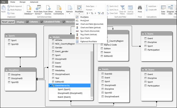
Click the PivotTable tab on the Ribbon in the Power Pivot window.
-
Click PivotTable on the Ribbon.
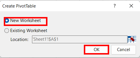
The Create PivotTable dialog box appears. Select New Worksheet and click OK.
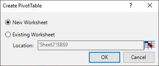
An empty PivotTable is created in a new worksheet.
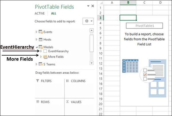
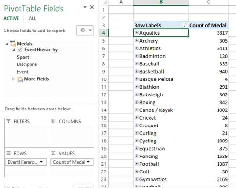
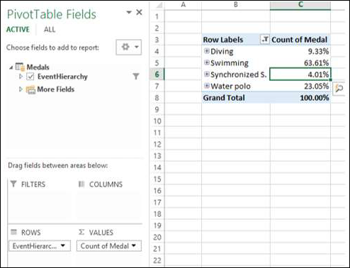
In the PivotTable Fields list, EventHierarchy appears as a field in Medals table. The other fields in the Medals table are collapsed and shown as More Fields.
-
Click on the arrow
in front of EventHierarchy. -
Click on the arrow
in front of More Fields.
The fields under EventHierarchy will be displayed. All the fields in the Medals table will be displayed under More Fields.
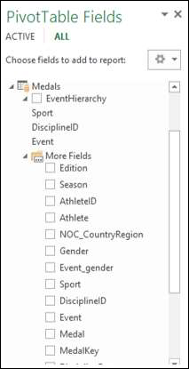
As you can observe, the three fields that you added to the hierarchy also appear under More Fields with check boxes. If you do not want them to appear in the PivotTable Fields list under More Fields, you have to hide the columns in the data table – Medals in data view in Power Pivot Window. You can always unhide them whenever you want.
Add fields to the PivotTable as follows −
-
Drag EventHierarchy to ROWS area.
-
Drag Medal to ∑ VALUES area.
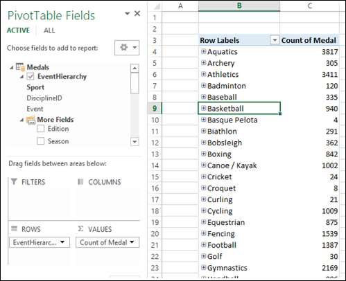
The values of Sport field appear in the PivotTable with a + sign in front of them. The medal count for each sport is displayed.
-
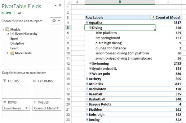
Click on the + sign before Aquatics. The DisciplineID field values under Aquatics will be displayed.
-
Click on the child D22 that appears. The Event field values under D22 will be displayed.
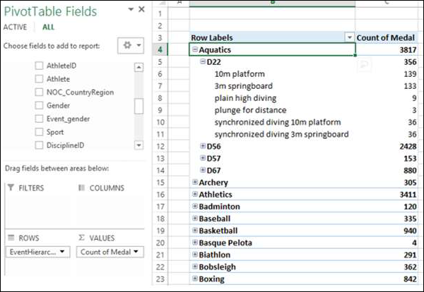
As you can observe, medal count is given for the Events, that get summed up at the parent level − DisciplineID, that get further summed up at the parent level − Sport.
Creating a Hierarchy based on Multiple Tables
Suppose you want to display the Disciplines in the PivotTable rather than DisciplineIDs to make it a more readable and understandable summarization. In order to do this, you need to have the field Discipline in Medals table that as you know is not. Discipline field is in Disciplines data table, but you cannot create a hierarchy with fields from more than one table. But, there is a way to obtain the required field from the other table.
As you are aware, the tables − Medals and Disciplines are related. You can add the field Discipline from Disciplines table to the Medals table, by creating a column using the relationship with DAX.
-
Click data view in Power Pivot window.
-
Click the Design tab on the Ribbon.
-
Click Add.
The column − Add Column on the right side of the table is highlighted.
Type = RELATED (Disciplines [Discipline]) in the formula bar. A new column − CalculatedColumn1 is created with the values as Discipline field values in the Disciplines table.
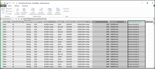
Rename the new column thus obtained in the Medals table as Discipline. Next, you have to remove DisciplineID from the Hierarchy and add Discipline, which you will learn in the following sections.
Removing a Child Level from a Hierarchy
As you can observe, the hierarchy is visible in the diagram view only, and not in the data view. Hence, you can edit a hierarchy in the diagram view only.
-
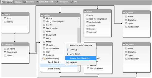
Click on the diagram view in the Power Pivot window.
-
Right click DisciplineID in EventHierarchy.
-
Select Remove from Hierarchy from the dropdown list.
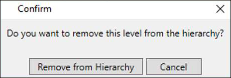
The Confirm dialog box appears. Click Remove from Hierarchy.
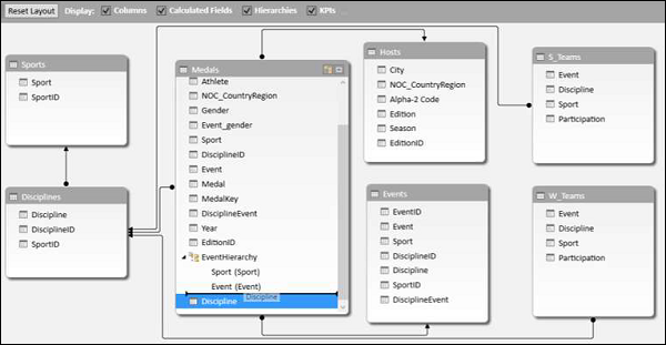
The field DisciplineID gets deleted from the hierarchy. Remember that you have removed the field from hierarchy, but the source field still exists in the data table.
Next, you need to add Discipline field to EventHierarchy.
Adding a Child Level to a Hierarchy
You can add the field Discipline to the existing hierarchy — EventHierarchy as follows −
-
Click on the field in Medals table.
-
Drag it to the Events field below in the EventHierarchy.
The Discipline field gets added to EventHierarchy.

As you can observe, the order of the fields in EventHierarchy is Sport–Event–Discipline. But, as you are aware it has to be Sport–Discipline-Event. Hence, you need to change the order of the fields.
Changing the Order of a Child Level in a Hierarchy
To move the field Discipline to the position after the field Sport, do the following −
-
Right click on the field Discipline in EventHierarchy.
-
Select Move Up from the dropdown list.
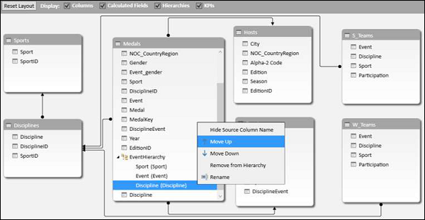
The order of the fields changes to Sport-Discipline-Event.
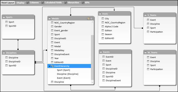
PivotTable with Changes in Hierarchy
To view the changes that you made in EventHierarchy in the PivotTable, you need not create a new PivotTable. You can view them in the existing PivotTable itself.
Click on the worksheet with the PivotTable in Excel window.
As you can observe, in the PivotTable Fields list, the child levels in the EventHierarchy reflect the changes you made in the Hierarchy in Data Model. The same changes also get reflected in the PivotTable accordingly.
Click the + sign in front of Aquatics in the PivotTable. The child levels appear as values of the field Discipline.
Hiding and Showing Hierarchies
You can choose to hide the Hierarchies and show them whenever you want.
-
Uncheck the box Hierarchies in the top menu of diagram view to hide the hierarchies.
-
Check the box Hierarchies to show the hierarchies.

Creating a Hierarchy in Other Ways
In addition to the way you created hierarchy in the previous sections, you can create a hierarchy in another two ways.
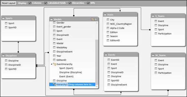
1. Click the Create Hierarchy button on the top right corner of the Medals data table in diagram view.
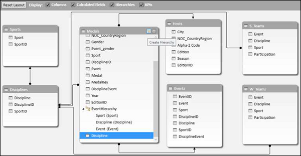
A new hierarchy gets created in the table without any fields in it.
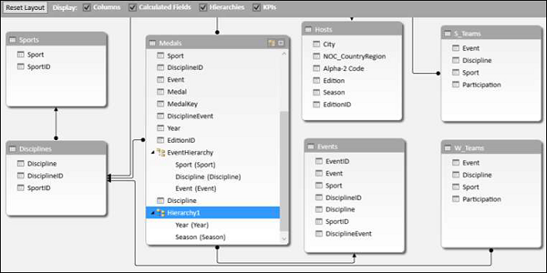
Drag the fields Year and Season, in that order to the new hierarchy. The hierarchy shows the child levels.
2. Another way of creating the same hierarchy is as follows −
-
Right click on the field Year in the Medals data table in diagram view.
-
Select Create Hierarchy from the dropdown list.
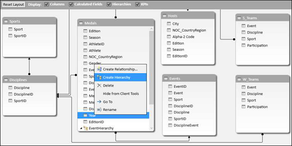
A new hierarchy is created in table with Year as a child field.
Drag the field season to the hierarchy. The hierarchy shows the child levels.

Deleting a Hierarchy
You can delete a hierarchy from the Data Model as follows −
-
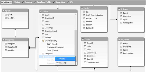
Right click on the hierarchy.
-
Select Delete from the dropdown list.
The Confirm dialog box appears. Click Delete from Model.
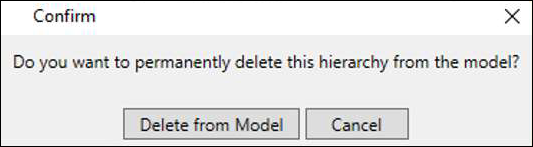
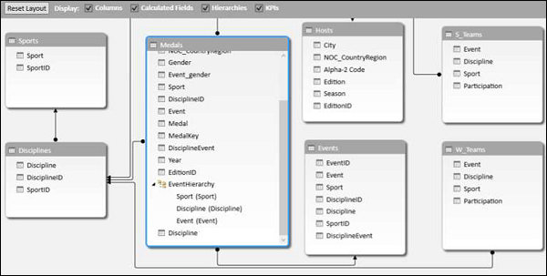
The hierarchy gets deleted.
Calculations Using Hierarchy
You can create calculations using a hierarchy. In the EventsHierarchy, you can display the number of medals at a child level as a percentage of the number of medals at its parent level as follows −
-
Right click on a Count of Medal value of an Event.
-
Select Value Field Settings from the dropdown list.
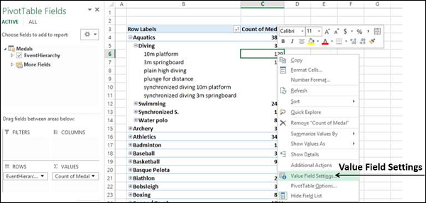
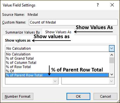
Value Field Settings dialog box appears.
-
Click the Show Values As tab.
-
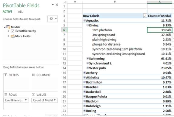
Select % of Parent Row Total from the list and click OK.
The child levels are displayed as the percentage of the Parent Totals. You can verify this by summing up the percentage values of the child level of a parent. The sum would be 100%.
Drilling Up and Drilling Down a Hierarchy
You can quickly drill up and drill down across the levels in a hierarchy using Quick Explore tool.
-
Click on a value of Event field in the PivotTable.
-
Click the Quick Explore tool —
that appears at the bottom right corner of the cell containing the selected value.
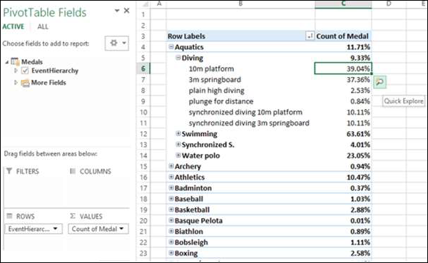
The Explore box with Drill Up option appears. This is because from Event you can only drill up as there are no child levels under it.
Click Drill Up.
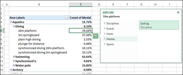
PivotTable data is drilled up to Discipline.
Click on the Quick Explore tool —  that appears at the bottom right corner of the cell containing a value.
Explore box appears with Drill Up and Drill Down options displayed. This is because from Discipline you can drill up to Sport or drill down to Event.

This way you can quickly move up and down the hierarchy.
A Hierarchy is a system that has many levels from highest to lowest. When we have related columns in a table, then analyzing them with fixed attributes is difficult. Excel Power Pivot gives us the power to set a hierarchy to which data can be filtered and analyzed correctly according to one’s needs. In this article, we will learn how to create hierarchies in the Power pivot.
Meaning of Hierarchy in Power Pivot
Hierarchy in a data set helps analyze complex data easily. A hierarchy is a list of nested columns in a table. Power Pivot hierarchies provide additional features and functionalities to help classify and analyze data efficiently. Hierarchy helps provide a large amount of data in a space-efficient manner. Power pivot hierarchies have aggregate functions like Count, Min, Max, Average, and Distinct Count, which help analyze different aspects of the data. One can also move to different levels in the hierarchy by the drill up and drill down option provided by PivotTableAnalyze. For example, Department, Project, and Employee all three columns can be combined into a single column as a hierarchy.
Creating a Hierarchy By Power Pivot
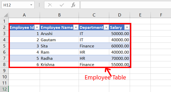
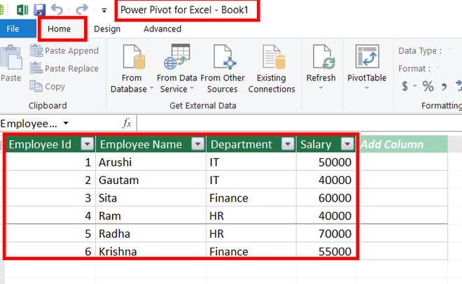
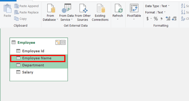
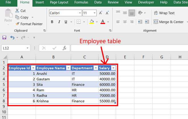
Given a data set, with a table in an excel sheet name Employee. The Attributes of the table are Employee Id, Employee Name, Department, and Salary. We need to create a hierarchy of Department ⇢ Employee Name providing Salary as values. Save the given excel sheet with employee.xlsx.
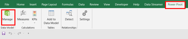
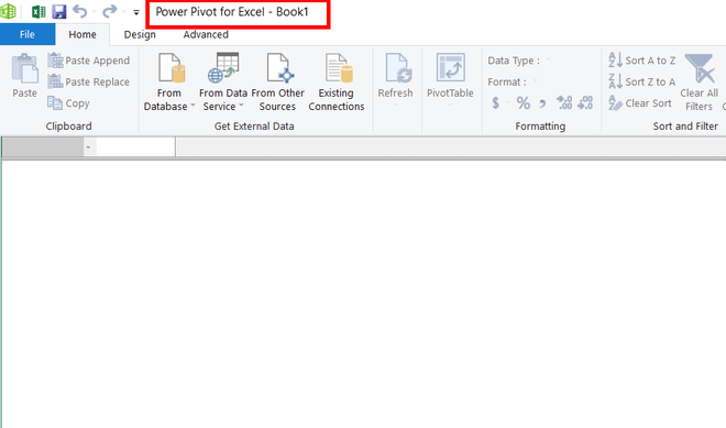
Step 1: Open a new blank sheet. Go to Power Pivot, and click on Manage.
Step 2: A new window name Power Pivot for Excel is opened.
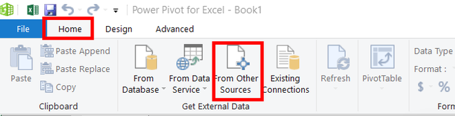
Step 3: Go to the Home tab. Under the Get External Data section, click on From Other Sources.
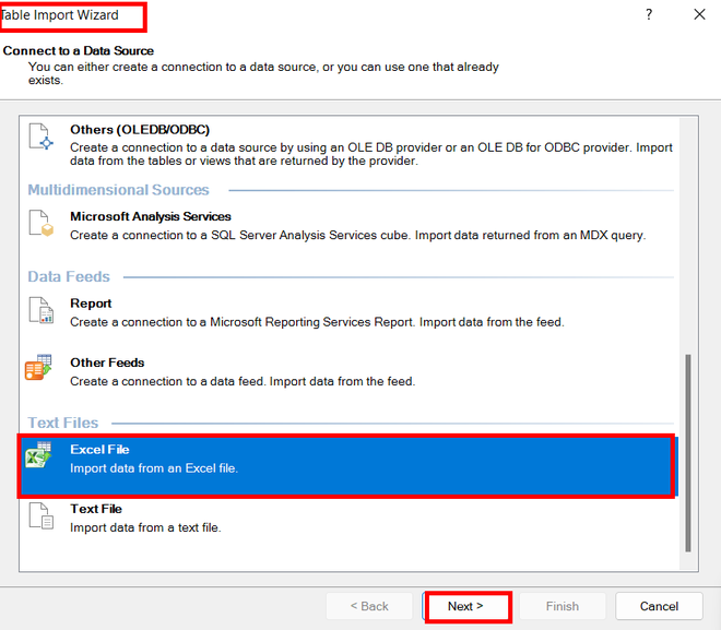
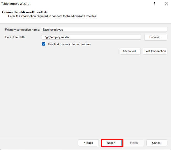
Step 4: A new window name Table import Wizard is opened. Under Text Files. Select Excel Files option. Click on Next.
Step 5: Firstly, check the box, Use First Row as column headers. Then, click on Browse.
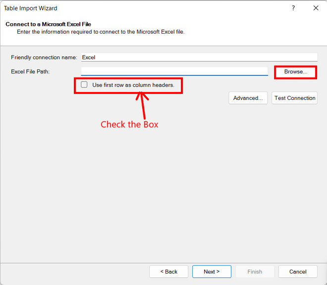
Step 6: Select the file employee.xlsx. Click on Ok.
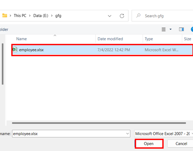
Step 7: The desired file is selected. Click on the Next button.
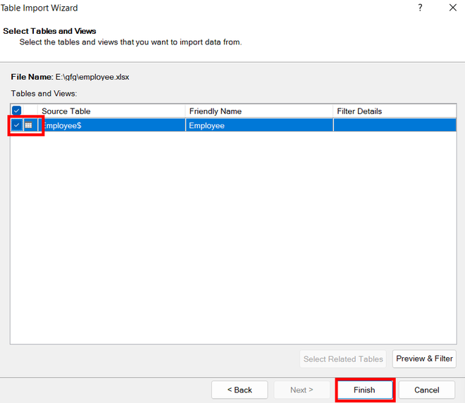
Step 8: Select the tables that you want to add to your power pivot. Click on the Finish button.
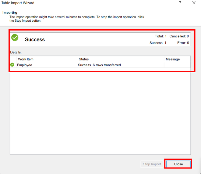
Step 9: The files will be imported and a success pane will appear. Click on the Close button.
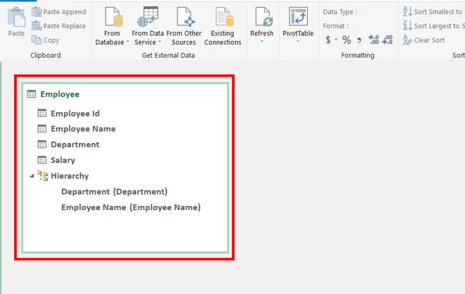
Step 10: Power Pivot window reappears. A table is inserted in your Power Pivot.
Step 11: Now, go to the Home tab. Under the view section, click on the Diagram View.
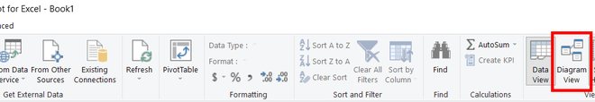
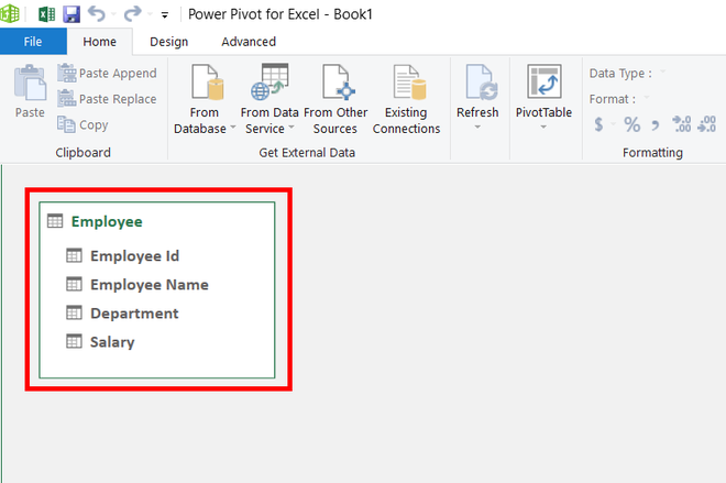
Step 12: The diagram view of the table appears with the names of the attributes.
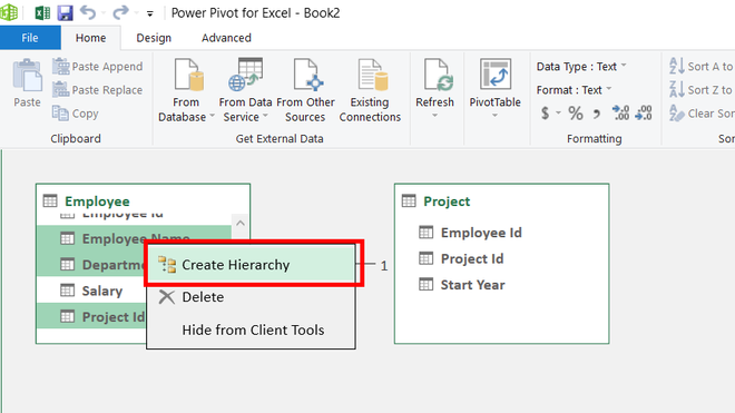
Step 13: Select the attributes you want in your hierarchy. For example, Department. The order in which you select the hierarchy is important, as the attribute selected first will appear at a higher level than the later selected attribute.
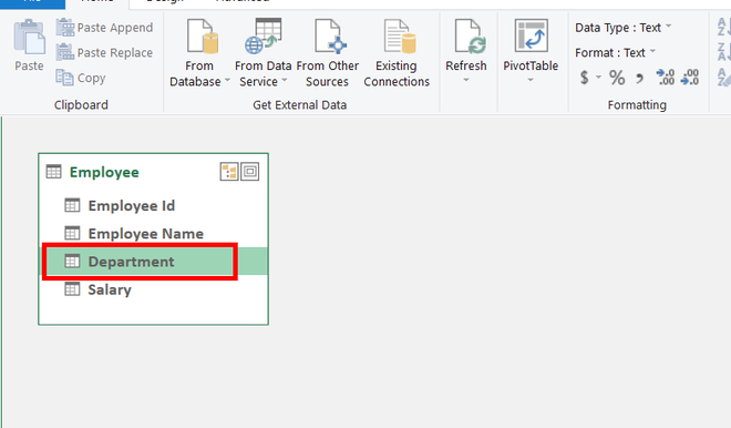
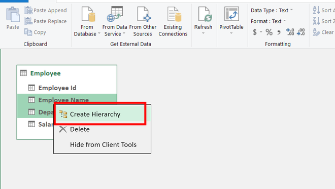
Step 14: To select multiple attributes, press Ctrl + mouse click.
Step 15: After selecting the desired attributes. Right-click on the Create Hierarchy.
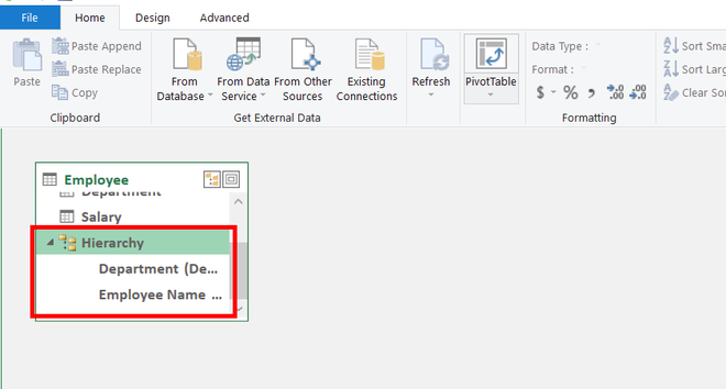
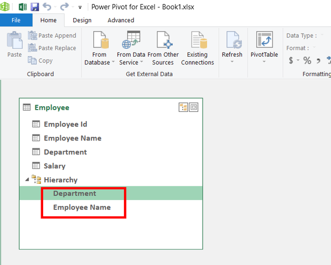
Step 16: A new attribute is created. Rename the attribute to your choice. For example, renaming the new attribute to Hierarchy.
Step 17: Go to the Home tab. Select PivotTable.
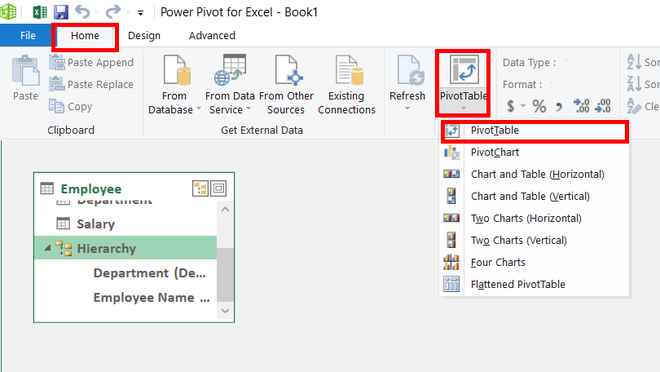
Step 18: A Create PivotTable dialogue box appears. Select the radio button, new worksheet, and click on Ok.
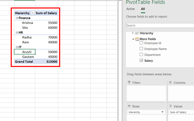
Step 19: PivotTable Fields appear on the right-most side of the worksheet.
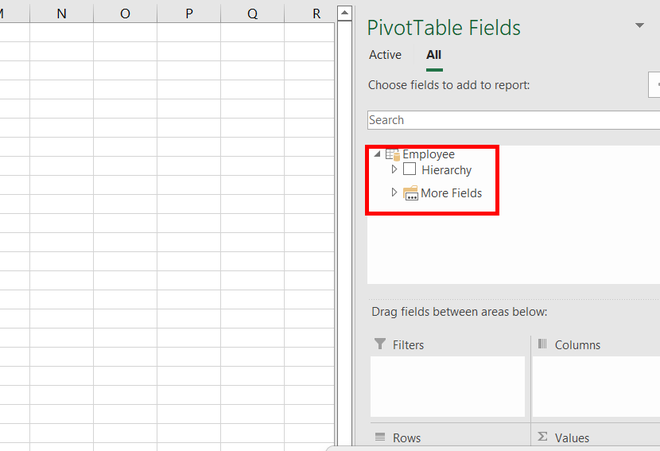
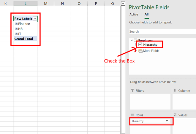
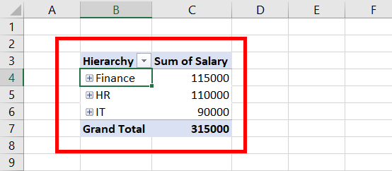
Step 20: Drag and Drop Hierarchy to Rows. A table with the highest level hierarchy appears.
Step 21: Drag and Drop Salary to Values.
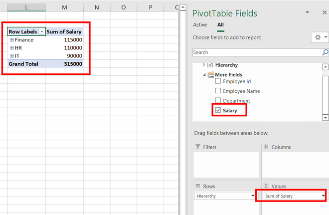
Step 22: A Hierarchy table is created. You can click on the + button, to move down to the next level in the hierarchy.
Exploring Different Features in Power Pivot Hierarchy
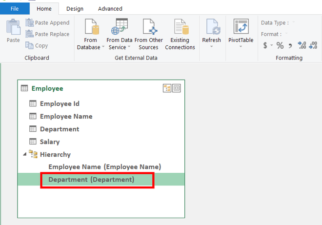
Now, we will explore different features in the hierarchy offered by the power pivot. Consider the hierarchy created above. i.e. Department ⇢ Employee Name.
- Changing the order in a Hierarchy
Given the Drawing View of the Employee Table.
Use Move Up and Move Down buttons to change the order of your hierarchy.
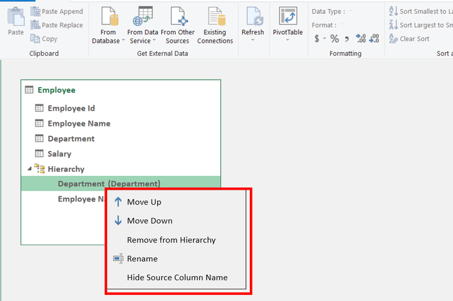
Step 1: Select any attribute in the hierarchy. For example, Department. Right-click on it.
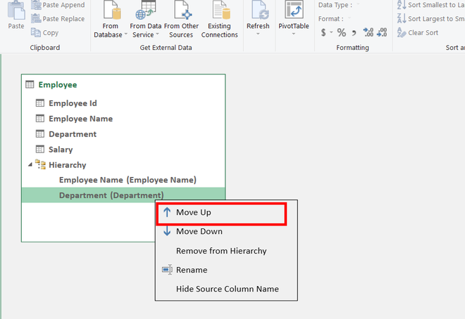
Step 2: Click on the Move Down button.
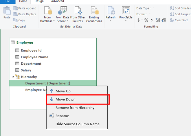
Step 3: This moves your attribute in the hierarchy to one level down. For example, the Department attribute comes under the Employee Name now.
Step 4: Again, Right-click on the Department. Click on the Move Up button.
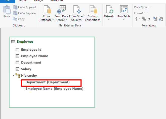
Step 5: The Move Up button moves your attribute to one level up in the hierarchy. For example, the Employee Name attribute comes under the Department now.
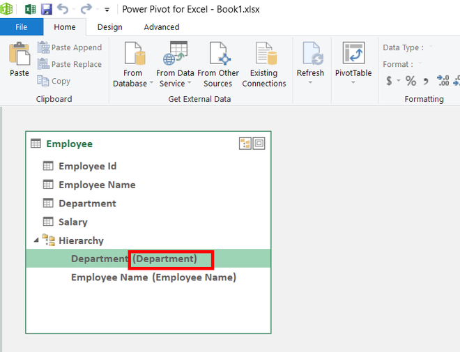
- Hiding or Showing Source column name in the Hierarchy
Given the Drawing View of the Employee table.
The Source Column Name can be different from the name in the Hierarchy.
Step 1: The text written in the Parenthesis is the Source Column Name. By default, the Source Column Name and the Hierarchy Column Name are the same.
Step 2: Right-Click on any attribute of the hierarchy attribute. Click on the Hide Source Column Name.
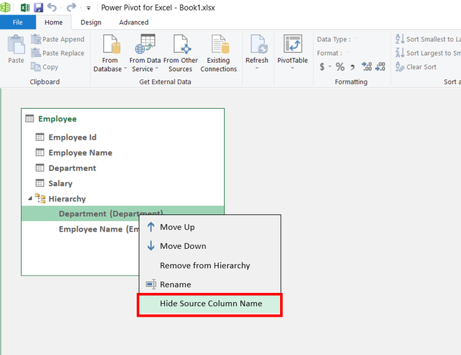
Step 3: The text is written in the parenthesis disappears.
- Drill Up and Drill Down in the Hierarchy
Consider the Hierarchical Pivot table created above.
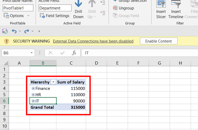
Drill Up and Drill down are used to come down or up a level in the hierarchy.
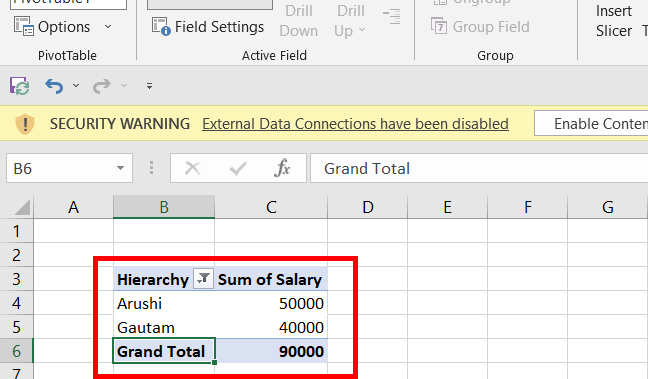
Step 1: Select cell B6 in the hierarchical pivot table. The department is IT.
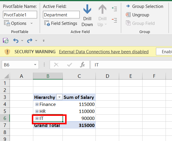
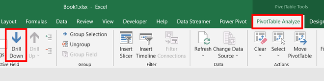
Step 2: Go to the PivotTable Analyze tab. Click on the Drill Down button.
Step 3: Now, the name of the employees will appear, working in that department. The selected cell moves down to one level.
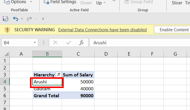
Step 4: To Drill Up in the table. Select any cell in the Hierarchy attribute. For example, select cell B4 i.e. Arushi.
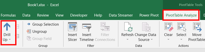
Step 5: Click on the Drill Up button.
Step 6: The table reaches back to its previous level.
Create An Hierarchy using In related Tables
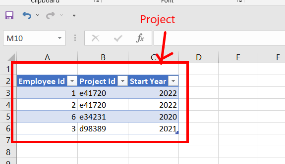
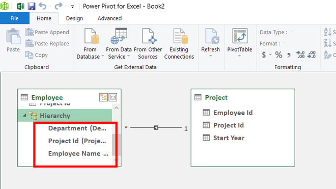
Creating Hierarchy between multiple tables is not possible in Power pivot. To add attributes of another table in your parent table can only be achieved if you add that attribute from another table to your parent table. Given a data set of two tables, one named Employee and the second named Project in two different excel sheets in the same workbook. For example, create a hierarchy of Department ⇢ Project Id ⇢ Employee Name. As Project Id is not present in the Employee table so we will add the Project Id attribute from the Project table to the Employee table.
Step 1: Create a Drawing view, of both the tables in the power pivot window, by importing the file in the power pivot window.
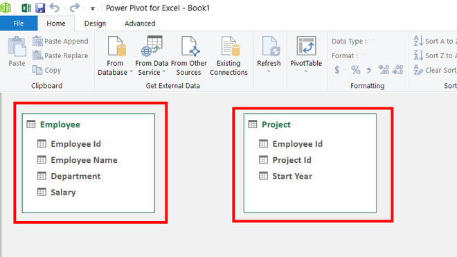
Step 2: Now, create a relation between the Employee table and the Project table. To do this, there should be at least one attribute common in both of the tables. Keep your cursor on the Employee table, select any attribute and drag the mouse to the Project table, leave your mouse click.
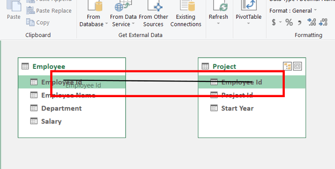
Step 3: A small arrow line is created between the tables, showing that both tables are related.
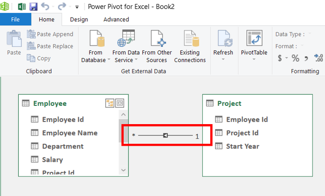
Step 4: Go to the Home tab, and click on the Data view option.
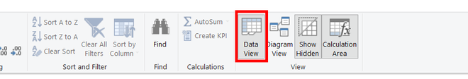
Step 5: Click on the Add Column.
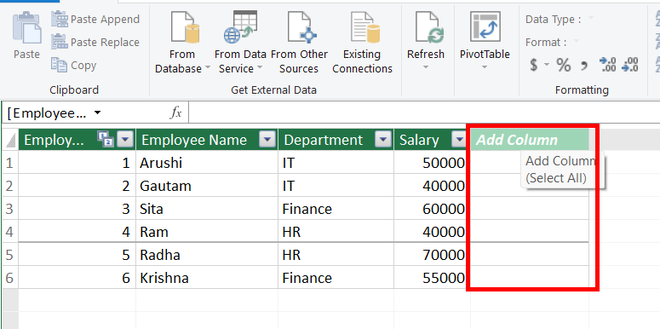
Step 6: Write a function =RELATED([Project Id]) in the ribbon. Press Enter.
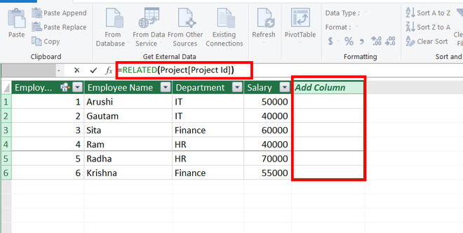
Step 7: A column name Calculated Column 1 is added to the Employee table.
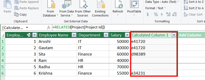
Step 8: Rename the attribute as Project Id.
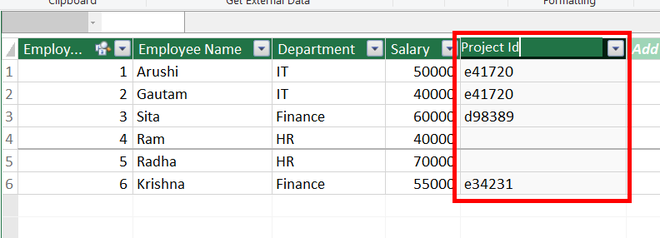
Step 9: Go to the Home tab, and click on the Draw View. Select the Attributes in the hierarchical order to be created i.e. Department ⇢ Project Id ⇢ Employee Name. Click on the Create Hierarchy.
Step 10: A Hierarchy is created.
|
Werty Пользователь Сообщений: 227 |
Здравствуйте, знатоки Excel! Подскажите пожалуйста, можно ли столбцы сводной расположить не вложенными друг в друга, а на одном уровне иерархии? Спокойствие — величайшее проявление силы. |
|
Werty
Изменено: Constantinich — 29.03.2017 10:26:19 |
|
|
Werty Пользователь Сообщений: 227 |
Здравствуйте! Ваш пример работает на область строк. Мой вопрос про область Столбцов. Спокойствие — величайшее проявление силы. |
|
Werty, не совсем понятно как это должно работать. Можете пример показать в таблице как это должно быть заполнено? Изменено: Constantinich — 28.03.2017 20:14:46 |
|
|
Werty Пользователь Сообщений: 227 |
да, уже делаю … Прикрепленные файлы
Изменено: Werty — 29.03.2017 10:26:33 Спокойствие — величайшее проявление силы. |
|
Werty Пользователь Сообщений: 227 |
Так, пример выложил, народ пропал Спокойствие — величайшее проявление силы. |
|
Андрей VG  Пользователь Сообщений: 11878 Excel 2016, 365 |
Доброе время суток. |
|
Werty Пользователь Сообщений: 227 |
Тогда теряется возможность использовать структуру: схлапывать и раскрывать строчки Спокойствие — величайшее проявление силы. |
|
Z  Пользователь Сообщений: 6111 Win 10, MSO 2013 SP1 |
#9 29.03.2017 09:04:10
Традиционно — кому охота ломать голову над вашей очередной заморочкой, тем более, что вы не оговариваете возможные варианты — хочу так и не иначе… Прикрепленные файлы
«Ctrl+S» — достойное завершение ваших гениальных мыслей!.. |
||

|
Werty, так как вы хотите, сделать просто сводником нельзя. Как вариант, сделать 2 сводника с одинаковой частью строк, а фильтроваться единым срезом, который привязан к 2-м сводникам Посмотрите во вложении |
|
|
Z Пользователь Сообщений: 6111 Win 10, MSO 2013 SP1 |
Избавитесь от «пустоты» — получите — «Ctrl+S» — достойное завершение ваших гениальных мыслей!.. |
|
Werty Пользователь Сообщений: 227 |
#12 29.03.2017 09:39:56
Здравствуйте, Z! Удобно это как?
Кому адресуете предложение?
Может быть я ошибаюсь и это не специализированный форум по Excel? Если я не ошибаюсь здесь все со своими «заморочками» обращаются. Спокойствие — величайшее проявление силы. |
||||||
|
Werty Пользователь Сообщений: 227 |
#13 29.03.2017 09:45:47
Посмотрел. Спасибо. Интересный финт Спокойствие — величайшее проявление силы. |
||
|
Z Пользователь Сообщений: 6111 Win 10, MSO 2013 SP1 |
#14 29.03.2017 09:52:48
OFF И тут он стабильно неповторим/неизменен: понимайте как хотите — плохо/хорошо, да/нет… Прощайте, Werty! «Ctrl+S» — достойное завершение ваших гениальных мыслей!.. |
||
|
Андрей VG Пользователь Сообщений: 11878 Excel 2016, 365 |
#15 29.03.2017 10:06:47
Работать будет до первой сортировки для примера , но в любом случае ассиметричные итоги могут быть только справа (учитывая ориентацию предложенного формата вывода). |
||
|
Werty Пользователь Сообщений: 227 |
Андрей, спасибо. Спокойствие — величайшее проявление силы. |
|
vikttur Пользователь Сообщений: 47199 |
#17 29.03.2017 10:29:57 Werty, не стоит иголки распускать. |
|
Группа: Пользователи Ранг: Прохожий Сообщений: 8
Замечаний: |

Добрый день!
Сразу несколько вопросов по сводной таблице (из вложения): 1) как сделать, чтобы номеру платежки соответствовала дата на том же уровне иерархии в названии строк, т.е. чтобы они отображались так, как если бы были в одной ячейке. Тем самым не дупуская повторений в полях значений; 2) чтобы при изменении данных в фильтре отчета, ширина столбцов оставалась постоянной.
К сообщению приложен файл:
4775258.xlsx
(16.6 Kb)