
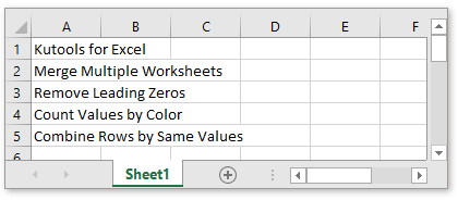
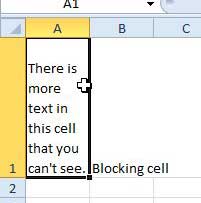
In Excel, sometimes, the cell contents are too many to display fully in the cell as below screenshot shown. Here in this tutorial, it provides some ways to display all content in a cell for users in Excel.
Display all contents with Wrap Text function
Display all contents with AutoFit Column Width function
Display all contents with Enhanced Edit Bar
Display all contents with Wrap Text function
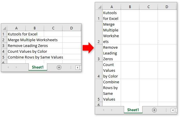
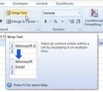
In Excel, the Wrap Text function will keep the column width and adjust the row height to display all contents in each cell.
Select the cells that you want to display all contents, and click Home > Wrap Text.
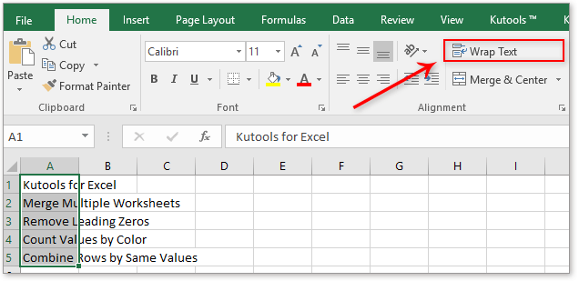
Then the selected cells will be expanded to show all contents.
Display all contents with AutoFit Column Width function
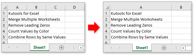
If you do not want to change the row heights of cells, you can use the AutoFit Column Width function to adjust the column width of cells for showing all contents.
Select the cells that you use, and click Home > Format > AutoFit Column Width.

Then the cells will be adjusted the column width for displaying the cell contents.
Display all contents with Enhanced Edit Bar
If there are large of contents in cells which you do not want to change the row height and column width of cells for keeping good-look of the worksheet, you can view all contents by using Kutools for Excel’s Enhanced Edit Bar function, which can display all contents in a prompt dialog while you click at the cell.
After free installing Kutools for Excel, please do as below:
Click Kutools > Enhanced Edit Bar to enable the Enhanced Edit Bar.

From now on, while you click at a cell, a dialog will prompt to display all contents of the active cell, and also, you can edit contents in this dialog directly to update contents in the cell.

Other Operations (Articles) Related To Text
Convert date stored as text to date in Excel
Occasionally, when you copy or import dates from other data sources to Excel cell, the date might become formatted and stored as texts. And here I introduce the tricks to convert such these dates stored as texts to standard dates in Excel.
Add text cells together into one cell in Excel
Sometimes, you need to combine text cells together into one cell in some purpose. In this article, we will show you two methods to add text cells together into one cell in Excel with details.
Allow only numbers to be input in text box
In Excel, we can apply the Data Validation function to allow only numbers to be entered into cells, but, sometimes, I want only numbers to be typed into a textbox as well as in cells. How to accept only numbers in a textbox in Excel?
Change case of text in Excel
This article is going to talk about the methods you can apply for changing text case easily in Excel.
The Best Office Productivity Tools
Kutools for Excel Solves Most of Your Problems, and Increases Your Productivity by 80%
- Super Formula Bar (easily edit multiple lines of text and formula); Reading Layout (easily read and edit large numbers of cells); Paste to Filtered Range…
- Merge Cells/Rows/Columns and Keeping Data; Split Cells Content; Combine Duplicate Rows and Sum/Average… Prevent Duplicate Cells; Compare Ranges…
- Select Duplicate or Unique Rows; Select Blank Rows (all cells are empty); Super Find and Fuzzy Find in Many Workbooks; Random Select…
- Exact Copy Multiple Cells without changing formula reference; Auto Create References to Multiple Sheets; Insert Bullets, Check Boxes and more…
- Favorite and Quickly Insert Formulas, Ranges, Charts and Pictures; Encrypt Cells with password; Create Mailing List and send emails…
- Extract Text, Add Text, Remove by Position, Remove Space; Create and Print Paging Subtotals; Convert Between Cells Content and Comments…
- Super Filter (save and apply filter schemes to other sheets); Advanced Sort by month/week/day, frequency and more; Special Filter by bold, italic…
- Combine Workbooks and WorkSheets; Merge Tables based on key columns; Split Data into Multiple Sheets; Batch Convert xls, xlsx and PDF…
- Pivot Table Grouping by week number, day of week and more… Show Unlocked, Locked Cells by different colors; Highlight Cells That Have Formula/Name…
")
Office Tab — brings tabbed interface to Office, and make your work much easier
- Enable tabbed editing and reading in Word, Excel, PowerPoint, Publisher, Access, Visio and Project.
- Open and create multiple documents in new tabs of the same window, rather than in new windows.
- Increases your productivity by 50%, and reduces hundreds of mouse clicks for you every day!
")
Comments (1)
No ratings yet. Be the first to rate!
Содержание
- How do I show all text in a cell?
- How do I show all text in a cell?
- Re: How do I show all text in a cell?
- Re: How do I show all text in a cell?
- Thread Information
- TEXT function
- Overview
- Download our examples
- Other format codes that are available
- Format codes by category
- Common scenario
- Frequently Asked Questions
How do I show all text in a cell?
LinkBack
Thread Tools
Rate This Thread
Display
How do I show all text in a cell?
I have copied (from an e-mail) and pasted a paragraph into a cell but not all
the text is showing (the cell has been formated to wrap text).
I have adjusted width/height, made sure the background was set to no fill,
all font is black and adjusted verticle & horizontal alignment. I even
unwrapped the text and merged a bunch a cells so that the text would show in
1 cell. This cut the text off as well but in a different spot. I have tried
all the obvious possible fixes but nothing has helped. Any suggestions?
Re: How do I show all text in a cell?
Merged cells do not hold any more text then any one original single cell.
Excel Help on «limits» or «specifications» reveals that Excel will allow
32,767 characters to be entered in a cell.
However, it goes on to state that «only 1024 characters will be visible or can
be printed»
To work around this limitation, stick a few ALT + ENTERs in at appropriate
spots, about every 100 characters..
The ALT + ENTER forces a line-feed and expands the 1024 limit.
How far is not really known. Just experiment.
. From Dave Peterson.
I put this formula in A1:
=»xxx»& REPT(REPT(«asdf «,25)&CHAR(10),58)&»yyy»
And adjusted the columnwidth, rowheight and font size and I got about 7300
characters to print ok.
Failing that, use a Text Box to store the text or MS Word which is a word
processing application, unlike Excel which is not.
Gord Dibben Excel MVP
On Wed, 19 Jul 2006 08:43:02 -0700, Rachel
wrote:
>I have copied (from an e-mail) and pasted a paragraph into a cell but not all
>the text is showing (the cell has been formated to wrap text).
>
>I have adjusted width/height, made sure the background was set to no fill,
>all font is black and adjusted verticle & horizontal alignment. I even
>unwrapped the text and merged a bunch a cells so that the text would show in
>1 cell. This cut the text off as well but in a different spot. I have tried
>all the obvious possible fixes but nothing has helped. Any suggestions?
>
Gord Dibben MS Excel MVP
Re: How do I show all text in a cell?
When text is long and just seems to fizzle out at the end, I add alt-enters
every 80-100 characters (yep, manually) to get it to display correctly.
And I sometimes have to set the rowheight manually.
Rachel wrote:
>
> I have copied (from an e-mail) and pasted a paragraph into a cell but not all
> the text is showing (the cell has been formated to wrap text).
>
> I have adjusted width/height, made sure the background was set to no fill,
> all font is black and adjusted verticle & horizontal alignment. I even
> unwrapped the text and merged a bunch a cells so that the text would show in
> 1 cell. This cut the text off as well but in a different spot. I have tried
> all the obvious possible fixes but nothing has helped. Any suggestions?
Thread Information
Users Browsing this Thread
There are currently 1 users browsing this thread. (0 members and 1 guests)
Источник
TEXT function
The TEXT function lets you change the way a number appears by applying formatting to it with format codes. It’s useful in situations where you want to display numbers in a more readable format, or you want to combine numbers with text or symbols.
Note: The TEXT function will convert numbers to text, which may make it difficult to reference in later calculations. It’s best to keep your original value in one cell, then use the TEXT function in another cell. Then, if you need to build other formulas, always reference the original value and not the TEXT function result.
The TEXT function syntax has the following arguments:
A numeric value that you want to be converted into text.
A text string that defines the formatting that you want to be applied to the supplied value.
Overview
In its simplest form, the TEXT function says:
=TEXT(Value you want to format, «Format code you want to apply»)
Here are some popular examples, which you can copy directly into Excel to experiment with on your own. Notice the format codes within quotation marks.
Currency with a thousands separator and 2 decimals, like $1,234.57. Note that Excel rounds the value to 2 decimal places.
Today’s date in MM/DD/YY format, like 03/14/12
Today’s day of the week, like Monday
Current time, like 1:29 PM
Percentage, like 28.5%
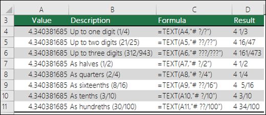
Fraction, like 4 1/3
Fraction, like 1/3. Note this uses the TRIM function to remove the leading space with a decimal value.
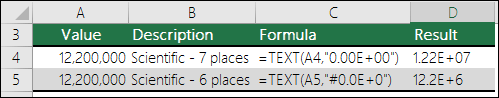
Scientific notation, like 1.22E+07
Add leading zeros (0), like 0001234
Note: Although you can use the TEXT function to change formatting, it’s not the only way. You can change the format without a formula by pressing CTRL+1 (or  +1 on the Mac), then pick the format you want from the Format Cells > Number dialog.
Download our examples
You can download an example workbook with all of the TEXT function examples you’ll find in this article, plus some extras. You can follow along, or create your own TEXT function format codes.
Other format codes that are available
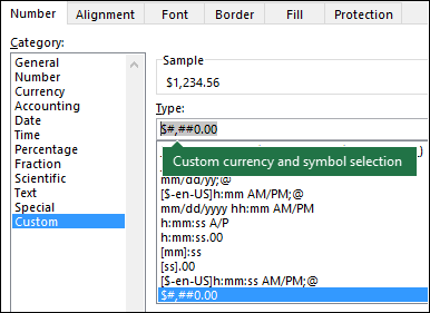
You can use the Format Cells dialog to find the other available format codes:
Press Ctrl+1 ( +1 on the Mac) to bring up the Format Cells dialog.
Select the format you want from the Number tab.
Select the Custom option,
The format code you want is now shown in the Type box. In this case, select everything from the Type box except the semicolon (;) and @ symbol. In the example below, we selected and copied just mm/dd/yy.
Press Ctrl+C to copy the format code, then press Cancel to dismiss the Format Cells dialog.
Now, all you need to do is press Ctrl+V to paste the format code into your TEXT formula, like: =TEXT(B2,» mm/dd/yy«). Make sure that you paste the format code within quotes («format code»), otherwise Excel will throw an error message.
 Cells > Number > Custom dialog to have Excel create format strings for you.» loading=»lazy»>
Format codes by category
Following are some examples of how you can apply different number formats to your values by using the Format Cells dialog, then use the Custom option to copy those format codes to your TEXT function.
Why does Excel delete my leading 0’s?
Excel is trained to look for numbers being entered in cells, not numbers that look like text, like part numbers or SKU’s. To retain leading zeros, format the input range as Text before you paste or enter values. Select the column, or range where you’ll be putting the values, then use CTRL+1 to bring up the Format > Cells dialog and on the Number tab select Text. Now Excel will keep your leading 0’s.
If you’ve already entered data and Excel has removed your leading 0’s, you can use the TEXT function to add them back. You can reference the top cell with the values and use =TEXT(value,»00000″), where the number of 0’s in the formula represents the total number of characters you want, then copy and paste to the rest of your range.
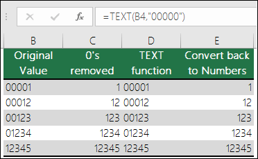
If for some reason you need to convert text values back to numbers you can multiply by 1, like =D4*1, or use the double-unary operator (—), like =—D4.
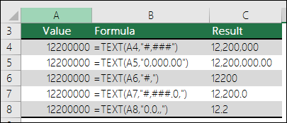
Excel separates thousands by commas if the format contains a comma (,) that is enclosed by number signs (#) or by zeros. For example, if the format string is «#,###», Excel displays the number 12200000 as 12,200,000.
A comma that follows a digit placeholder scales the number by 1,000. For example, if the format string is «#,###.0,», Excel displays the number 12200000 as 12,200.0.
The thousands separator is dependent on your regional settings. In the US it’s a comma, but in other locales it might be a period (.).
The thousands separator is available for the number, currency and accounting formats.
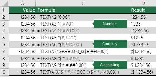
Following are examples of standard number (thousands separator and decimals only), currency and accounting formats. Currency format allows you to insert the currency symbol of your choice and aligns it next to your value, while accounting format will align the currency symbol to the left of the cell and the value to the right. Note the difference between the currency and accounting format codes below, where accounting uses an asterisk (*) to create separation between the symbol and the value.
To find the format code for a currency symbol, first press Ctrl+1 (or +1 on the Mac), select the format you want, then choose a symbol from the Symbol drop-down:
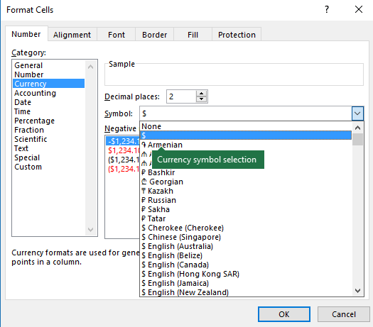
Then click Custom on the left from the Category section, and copy the format code, including the currency symbol.
Note: The TEXT function does not support color formatting, so if you copy a number format code from the Format Cells dialog that includes a color, like this: $#,##0.00_); [Red]($#,##0.00), the TEXT function will accept the format code, but it won’t display the color.
You can alter the way a date displays by using a mix of «M» for month, «D» for days, and «Y» for years.
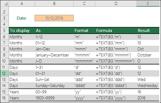
Format codes in the TEXT function aren’t case sensitive, so you can use either «M» or «m», «D» or «d», «Y» or «y».

If you share Excel files and reports with users from different countries, then you might want to give them a report in their language. Excel MVP, Mynda Treacy has a great solution in this Excel Dates Displayed in Different Languages article. It also includes a sample workbook you can download.
You can alter the way time displays by using a mix of «H» for hours, «M» for minutes, or «S» for seconds, and «AM/PM» for a 12-hour clock.
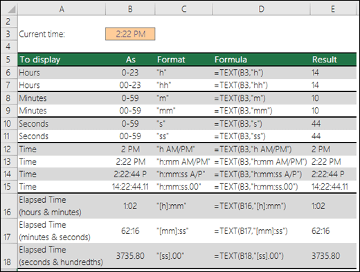
If you leave out the «AM/PM» or «A/P», then time will display based on a 24-hour clock.
Format codes in the TEXT function aren’t case sensitive, so you can use either «H» or «h», «M» or «m», «S» or «s», «AM/PM» or «am/pm».
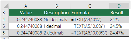
You can alter the way decimal values display with percentage (%) formats.
You can alter the way decimal values display with fraction (?/?) formats.
Scientific notation is a way of displaying numbers in terms of a decimal between 1 and 10, multiplied by a power of 10. It is often used to shorten the way that large numbers display.
Excel provides 4 special formats:
Zip Code — «00000»
Zip Code + 4 — «00000-0000»
Social Security Number — «000-00-0000»
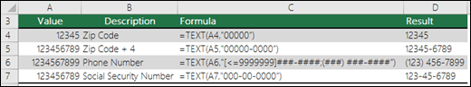
Special formats will be different depending on locale, but if there aren’t any special formats for your locale, or if these don’t meet your needs then you can create your own through the Format Cells > Custom dialog.
Common scenario
The TEXT function is rarely used by itself, and is most often used in conjunction with something else. Let’s say you want to combine text and a number value, like “Report Printed on: 03/14/12”, or “Weekly Revenue: $66,348.72”. You could type that into Excel manually, but that defeats the purpose of having Excel do it for you. Unfortunately, when you combine text and formatted numbers, like dates, times, currency, etc., Excel doesn’t know how you want to display them, so it drops the number formatting. This is where the TEXT function is invaluable, because it allows you to force Excel to format the values the way you want by using a format code, like «MM/DD/YY» for date format.
In the following example, you’ll see what happens if you try to join text and a number without using the TEXT function. In this case, we’re using the ampersand ( &) to concatenate a text string, a space (» «), and a value with =A2&» «&B2.
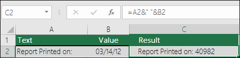
As you can see, Excel removed the formatting from the date in cell B2. In the next example, you’ll see how the TEXT function lets you apply the format you want.
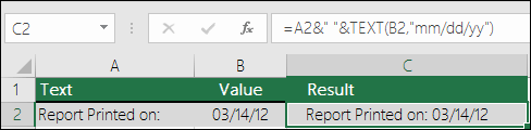
Our updated formula is:
Cell C2: =A2&» «&TEXT(B2,»mm/dd/yy») — Date format
Frequently Asked Questions
Unfortunately, you can’t do that with the TEXT function, you need to use Visual Basic for Applications (VBA) code. The following link has a method: How to convert a numeric value into English words in Excel
Yes, you can use the UPPER, LOWER and PROPER functions. For example, =UPPER(«hello») would return «HELLO».
Yes, but it takes a few steps. First, select the cell or cells where you want this to happen and use Ctrl+1 to bring up the Format > Cells dialog, then Alignment > Text control > check the Wrap Text option. Next, adjust your completed TEXT function to include the ASCII function CHAR(10) where you want the line break. You might need to adjust your column width depending on how the final result aligns.
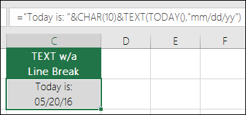
In this case, we used: =»Today is: «&CHAR(10)&TEXT(TODAY(),»mm/dd/yy»)
This is called Scientific Notation, and Excel will automatically convert numbers longer than 12 digits if a cell(s) is formatted as General, and 15 digits if a cell(s) is formatted as a Number. If you need to enter long numeric strings, but don’t want them converted, then format the cells in question as Text before you input or paste your values into Excel.
If you share Excel files and reports with users from different countries, then you might want to give them a report in their language. Excel MVP, Mynda Treacy has a great solution in this Excel Dates Displayed in Different Languages article. It also includes a sample workbook you can download.
Источник
Содержание
- 1 Перенос текста в ячейке Excel
- 1.1 Понравилась статья — нажмите на кнопки:
- 2 Способ 1
- 3 Способ 2
- 4 Способ 3
- 5 Способ 4
- 6 Способ 5
- 7 Excel длина текста в ячейке
09:53
Людмила
Просмотров: 20553
Перенос текста в ячейке Excel. Ни одна таблица не обходится без текста. Текст в рабочей таблице используется в основном для заголовков и различных спецификаций и примечаний. В Excel текст выравнивается по левому краю ячеек. Если текст длинный и не умещается в одной ячейке, то он выходит за её пределы и занимает пространство соседних клеток с правой стороны. Но как только вы введете какое-то значение или текст в соседние клетки, то остальная часть текста, которая находилась в предыдущей клетке становиться не видна. Для того, что бы в ячейке отображался весь текст необходимо либо раздвинуть ячейку с длинным текстом (что не всегда удобно), либо сделать перенос текста в ячейке Excel.
Для этого щелкните правой кнопкой мыши по ячейке, в которой находится начало вашего текста, и в выпадающем списке выберите пункт Формат ячеек.

В открывшемся окне Формат ячеек выберите вкладку Выравнивание и установите галочку на функцию Переносить по словам.

Не забудьте подтвердить свои изменения, нажав кнопку ОК.

Вот вы и сделали перенос текста в ячейке Excel . Теперь весь ваш длинный текст будет полностью виден в одной ячейке.
Этот метод подходит для всех версий Excel.
Посмотрите видеоролик Перенос текста в ячейке Excel:
С уважением, Людмила
Понравилась статья — нажмите на кнопки:
Если Вы периодически создаете документы в программе Microsoft Excel, тогда заметили, что все данные, которые вводятся в ячейку, прописываются в одну строчку. Поскольку это не всегда может подойти, и вариант растянуть ячейку так же не уместен, возникает необходимость переноса текста. Привычное нажатие «Enter» не подходит, поскольку курсор сразу перескакивает на новую строку, и что делать дальше?
Вот в этой статье мы с Вами и научимся переносить текст в Excel на новую строку в пределах одной ячейки. Рассмотрим, как это можно сделать различными способами.
Способ 1
Использовать для этого можно комбинацию клавиш «Alt+Enter». Поставьте курсив перед тем словом, которое должно начинаться с новой строки, нажмите «Alt», и не отпуская ее, кликните «Enter». Все, курсив или фраза перепрыгнет на новую строку. Напечатайте таким образом весь текст, а потом нажмите «Enter».

Выделится нижняя ячейка, а нужная нам увеличится по высоте и текст в ней будет виден полностью.
Чтобы быстрее выполнять некоторые действия, ознакомьтесь со списком горячих клавиш в Эксель.

Способ 2
Для того чтобы во время набора слов, курсив перескакивал автоматически на другую строку, когда текст уже не вмещается по ширине, сделайте следующее. Выделите ячейку и кликните по ней правой кнопкой мыши. В контекстном меню нажмите «Формат ячеек».

Вверху выберите вкладку «Выравнивание» и установите птичку напротив пункта «переносить по словам». Жмите «ОК».

Напишите все, что нужно, а если очередное слово не будет вмещаться по ширине, оно начнется со следующей строки.
Если в документе строки должны переноситься во многих ячейках, тогда предварительно выделите их, а потом поставьте галочку в упомянутом выше окне.
Способ 3
В некоторых случаях, все то, о чем я рассказала выше, может не подойти, поскольку нужно, чтобы информация с нескольких ячеек была собрана в одной, и уже в ней поделена на строки. Поэтому давайте разбираться, какие формулы использовать, чтобы получить желаемый результат.
Одна из них – это СИМВОЛ(). Здесь в скобках нужно указать значение от единицы до 255. Число берется со специальной таблицы, в которой указано, какому символу оно соответствует. Для переноса строчки используется код 10.
Теперь о том, как работать с формулой. Например, возьмем данные с ячеек A1:D2 и то, что написано в разных столбцах (A, B, C, D), сделаем в отдельных строчках.
Ставлю курсив в новую ячейку и в строку формул пишу:
=A1&A2&СИМВОЛ(10)&B1&B2&СИМВОЛ(10)&C1&C2&СИМВОЛ(10)&D1&D2
Знаком «&» мы сцепляем ячейки А1:А2 и так далее. Нажмите «Enter».

Не пугайтесь результата – все будет написано в одну строку. Чтобы это поправить, откройте окно «Формат ячеек» и поставьте галочку в пункте перенос, про это написано выше.

В результате, мы получим то, что хотели. Информация будет взята с указанных ячеек, а там, где было поставлено в формуле СИМВОЛ(10), сделается перенос.

Способ 4
Для переноса текста в ячейке используется еще одна формула – СЦЕПИТЬ(). Давайте возьмем только первую строку с заголовками: Фамилия, Долг, К оплате, Сумма. Кликните по пустой ячейке и введите формулу:
=СЦЕПИТЬ(A1;СИМВОЛ(10);B1;СИМВОЛ(10);C1;СИМВОЛ(10);D1)
Вместо A1, B1, C1, D1 укажите нужные Вам. Причем их количество можно уменьшить или увеличить.

Результат у нас получится такой.
Поэтому открываем уже знакомое окно Формата ячеек и отмечаем пункт переноса. Теперь нужные слова будут начинаться с новых строчек.

В соседнюю ячейку я вписала такую же формулу, только указала другие ячейки: A2:D2.
Плюс использования такого метода, как и предыдущего, в том, что при смене данных в исходных ячейках, будут меняться значения и в этих.
В примере изменилось число долга. Если еще и посчитать автоматически сумму в Экселе, тогда менять вручную больше ничего не придется.

Способ 5
Если же у Вас уже есть документ, в котором много написано в одной ячейке, и нужно слова перенести, тогда воспользуемся формулой ПОДСТАВИТЬ().

Суть ее в том, что мы заменим все пробелы на символ переноса строчки. Выберите пустую ячейку и добавьте в нее формулу:
=ПОДСТАВИТЬ(A11;» «;СИМВОЛ(10))
Вместо А11 будет Ваш исходный текст. Нажмите кнопку «Enter» и сразу каждое слово отобразится с новой строки.

Кстати, чтобы постоянно не открывать окно Формат ячеек, можно воспользоваться специальной кнопкой «Перенести текст», которая находится на вкладке «Главная».

Думаю, описанных способов хватит, чтобы перенести курсив на новую строку в ячейке Excel. Выбирайте тот, который подходит больше всего для решения поставленной задачи.
Поделитесь статьёй с друзьями:
Excel длина текста в ячейке
В разделе Программное обеспечение на вопрос Как в Excel сделать так, чтобы уместить текст в ячейке? заданный автором K лучший ответ это Выделяешь ячейку, правой кнопкой Формат ячейки, выравнивание, Поставить галочку переносить по словам
Ответ от
2 ответа
Привет! Вот подборка тем с ответами на Ваш вопрос: Как в Excel сделать так, чтобы уместить текст в ячейке?
Ответ от Добавляйтесь в друзья
Пиши все в одну строчку, а затем регулируй текст высотой и шириной строки
Ответ от |Аннушка|
EXEL НА ТО И EXEL,ЧТО В КАЖДОЙ ЯЧЕЙКЕ МОЖЕТ БЫТЬ ТОЛЬКО ОДНА СТРОКА
ТАК, КАК ХОЧЕШЬ СДЕЛАТЬ ТЫ, УВЫ, НЕВОЗМОЖНО
А ЕСЛИ ДЕЛАТЬ КАК YANA Цветочек ТО ПОТОМ БУДЕТ ВИДНА ТОЛЬКО ЧАСТЬ НАБРАННОГО ТЕКСТА
Ответ от Aristocratmodels@inbox.ru
Если у тебя длинный текст в 1 строку, а тебе надо, чтобы он в ячейке помещался в несколько строк, оставаясь в пределах ширины ячейки, делай, как говорит YANA Цветочек. Выдели все нужные ячейки, открой Формат — Выравнивание, поставь галочку «Переносить по словам», и у тебя ячейка сама будет раздвигаться вниз при переносе слова на следующую строку. .
А Аннушку не слушай.
Чтобы после нажатия Enter остаться в той же ячейке, а текст перешел на следующую строку, нажми Alt+Enter
Ответ от Ёергей Грачёв
Есть ешё способ.
Бывает, что нужно что бы перенос на другую строку был после конкретного слова, для этого после этого слова нажимаем сочетание клавиш «alt+enter»
Ответ от ???Prophet???
alt+enter»
Ответ от
2 ответа
Привет! Вот еще темы с нужными ответами:
Occasionally you will need to put a lot of data into a single cell in Excel. You may already know how to manually adjust the size of a cell to make that text visible, but this may not be the ideal solution for every situation. Excel has a “Wrap Text” feature that you can use to automatically adjust the size and appearance of a cell so that you can read all of the text contained within the cell.
Using Wrap Text in Excel 2010
Excel is automatically going to to determine the necessary row height for the information contained within your cell. The current column width will remain the same once you click the Wrap Text button. If you find that, after using the Wrap Text tool, you are not happy with the appearance of the data displayed inside the cell, you can manually increase the column width or the row height until you are happy.
Step 1: Open your spreadsheet in Excel 2010.
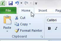
Step 2: Click the Home tab at the top of the window.
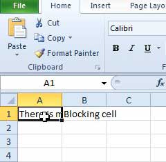
Step 3: Click the cell containing the text that you want to display.
Step 4: Click the Wrap Text button in the Alignment section of the ribbon at the top of the window.
All of the text inside the cell will now be visibly displayed on your spreadsheet.
As mentioned previously, you can manually resize the rows and columns as needed to improve the appearance of the text as well.
Everyone should be backing up their important pictures and files in case something happens to their computer or hard drive. One of the best ways to do this is with an external USB hard drive, which can be purchased at very affordable prices. Click here to check out a 1 TB option at Amazon.
Our article about how to fit a spreadsheet on one page in Excel 2010 offers an easy option to simplify Excel printing.

Matthew Burleigh has been writing tech tutorials since 2008. His writing has appeared on dozens of different websites and been read over 50 million times.
After receiving his Bachelor’s and Master’s degrees in Computer Science he spent several years working in IT management for small businesses. However, he now works full time writing content online and creating websites.
His main writing topics include iPhones, Microsoft Office, Google Apps, Android, and Photoshop, but he has also written about many other tech topics as well.
Read his full bio here.
07-19-2006, 11:50 AM
#1
How do I show all text in a cell?
I have copied (from an e-mail) and pasted a paragraph into a cell but not all
the text is showing (the cell has been formated to wrap text).I have adjusted width/height, made sure the background was set to no fill,
all font is black and adjusted verticle & horizontal alignment. I even
unwrapped the text and merged a bunch a cells so that the text would show in
1 cell. This cut the text off as well but in a different spot. I have tried
all the obvious possible fixes but nothing has helped. Any suggestions?
07-19-2006, 12:10 PM
#2
Re: How do I show all text in a cell?
Rachel
Merged cells do not hold any more text then any one original single cell.
Excel Help on «limits» or «specifications» reveals that Excel will allow
32,767 characters to be entered in a cell.However, it goes on to state that «only 1024 characters will be visible or can
be printed»To work around this limitation, stick a few ALT + ENTERs in at appropriate
spots, about every 100 characters..The ALT + ENTER forces a line-feed and expands the 1024 limit.
How far is not really known. Just experiment.
………From Dave Peterson……….
I put this formula in A1:
=»xxx»& REPT(REPT(«asdf «,25)&CHAR(10),58)&»yyy»And adjusted the columnwidth, rowheight and font size and I got about 7300
characters to print ok.………End Dave P……………..
Failing that, use a Text Box to store the text or MS Word which is a word
processing application, unlike Excel which is not.Gord Dibben Excel MVP
On Wed, 19 Jul 2006 08:43:02 -0700, Rachel <Rachel@discussions.microsoft.com>
wrote:
>I have copied (from an e-mail) and pasted a paragraph into a cell but not all
>the text is showing (the cell has been formated to wrap text).
>
>I have adjusted width/height, made sure the background was set to no fill,
>all font is black and adjusted verticle & horizontal alignment. I even
>unwrapped the text and merged a bunch a cells so that the text would show in
>1 cell. This cut the text off as well but in a different spot. I have tried
>all the obvious possible fixes but nothing has helped. Any suggestions?
>Gord Dibben MS Excel MVP
07-19-2006, 12:25 PM
#3
Re: How do I show all text in a cell?
When text is long and just seems to fizzle out at the end, I add alt-enters
every 80-100 characters (yep, manually) to get it to display correctly.And I sometimes have to set the rowheight manually.
Rachel wrote:
>
> I have copied (from an e-mail) and pasted a paragraph into a cell but not all
> the text is showing (the cell has been formated to wrap text).
>
> I have adjusted width/height, made sure the background was set to no fill,
> all font is black and adjusted verticle & horizontal alignment. I even
> unwrapped the text and merged a bunch a cells so that the text would show in
> 1 cell. This cut the text off as well but in a different spot. I have tried
> all the obvious possible fixes but nothing has helped. Any suggestions?—
Dave Peterson