Excel show all sheets on one sheet

The default setting in Excel is to show all the tabs (also called sheets) below the working area.

But if you can’t see any tabs and are wondering where has it disappeared, worry not. There are some possible reasons that may have been the cause of missing tabs in your Excel workbook.

In this article, I will show you a couple of methods you can use to restore the missing tabs in your Excel Workbook.

If you can’t see any of the tab names, it is most likely because of a setting that needs to be changed.

And in case you can see some of the sheet tabs but not all the sheet tabs, one possible reason could be that the sheets have been hidden, and you need to unhide the sheets to make the sheet tabs visible.

Another less likely but possible reason could be that the scrollbar he’s hiding the sheet tabs (when there are more sheets that extends beyond where the scrollbar starts)

Let’s have a look at each of these scenarios.

When All the Sheet Tabs are Missing

Whenever you open an Excel workbook, it must have at least one sheet tab in it (even if it’s a new blank workbook).

If you can’t see any tab, this most likely means that you need to change a setting that will enable the visibility of the tabs.

Below are the steps to restore the visibility of the tabs in Excel:

1. Click the File tab

1. Click on Options

1. In the ‘Options’ dialog box that opens, click on the Advanced option

1. Scroll down to the ‘Display Options for this Workbook’ section
2. Check the ‘Show sheet tabs’ option

The above change would ensure that all the available sheet tabs in the workbook become visible (unless the user has specifically hidden some of the worksheets)

Note that this setting is workbook specific – which means that in case you enable this setting in one of the workbooks, it would only make the tabs reappear in that specific workbook

When Some of the Sheet Tabs are Missing

Sometimes, you may be able to see some of the tabs in the workbook, while some others may be missing.

In this section, I have some solutions when only some of the tabs are missing and some are visible.

Some of the Sheets are Hidden

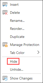
The most likely reason that you cannot see some of the tabs in the workbook is that they have been hidden by the user.

When a worksheet is hidden in Excel, it continues to exist as a part of the Excel workbook, but you don’t see that sheet tab name along with other sheet tabs.

And this has a really simple solution – you need to unhide the sheets.

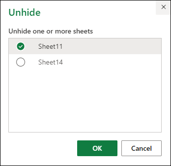
Below are the steps to unhide one or more sheets in Excel:

1. Right-click on any of the existing sheet tab name
2. Click on the Unhide option. In case there are no hidden sheets in the workbook, this option will be grayed out

1. In the Unhide dialog box, click on the sheet name you want to unhide

1. Click on OK

The above steps would unhide the selected sheet, and it would reappear as a tab in your workbook.

In case you want to unhide multiple sheets, you can select them in one go in the ‘Unhide’ dialog box. To do this, hold the Control key (or Command key if using Mac) and then click on the Sheet names that you want to unhide. This would select all the sheets on which you click and then you can unhide all these with one click.

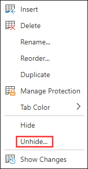
But what if you do not see the tab name in the names listed in the Unhide dialog box?

Well, there is a way in Excel to hide a sheet in such a way that its name doesn’t show up in the Unhide dialog box.

Then how do you unhide these ‘very hidden’ sheets?

You can read my tutorial here where I show you how to unhide those sheets that have been ‘very hidden’. It’s easy and it will only take a couple of clicks.

Tabs are Hidden Because of the Scroll Bar

Another reason your tabs may be missing could be because of a large scroll bar that hides the tabs.

And it has a simple fix – resize the scroll bar to make all other tabs visible.

Below I have a screenshot of an Excel workbook where I have 8 sheets but only three sheet tabs are visible. This is because of a large scrollbar that hides those tab names.

To get the sheet tabs to reappear, click on the three dots icon on the left of the scrollbar and drag it to the right. This will minimize the scroll bar and all the sheet tabs that were earlier hidden would now become visible.

In case you have a large workbook with a lot of sheets, even if you minimize the scrollbar, some sheet tabs would still be hidden.

In such a case, you can use the navigation icons (which are at the left of the first sheet tab) to make those sheet tabs visible.

So these are some of the ways you can use to fix the issue when the sheet tabs are missing and not showing in Excel. If you don’t see any sheet tab in the workbook, it’s most likely because of the setting in the Excel Options dialog box that needs to be changed.

And in case you see some sheet tab names but some are missing, then you need to check if some of the sheets have been hidden by the user or if they are hidden because of a large scroll bar.

Other Excel tutorials you may also like:

• Microsoft Excel Won’t Open – How to Fix it! (6 Possible Solutions)
• How to Switch Between Sheets in Excel? (7 Better Ways)
• Count Sheets in Excel (using VBA)
• How to Get the Sheet Name in Excel? Easy Formula
• How to Insert New Worksheet in Excel (Easy Shortcuts)
• How to Delete Sheets in Excel (Shortcuts + VBA)
• Arrow Keys not Working in Excel | Moving Pages Instead of Cells
• How to Change the Color of the Sheet Tab in Excel

Hide or unhide a worksheet

Note: The screen shots in this article were taken in Excel 2016. If you have a different version your view might be slightly different, but unless otherwise noted, the functionality is the same.

1. Select the worksheets that you want to hide.

   How to select worksheets

   To select	Do this
   A single sheet	Click the sheet tab. If you don’t see the tab that you want, click the scrolling buttons to the left of the sheet tabs to display the tab, and then click the tab.
   Two or more adjacent sheets	Click the tab for the first sheet. Then hold down Shift while you click the tab for the last sheet that you want to select.
   Two or more nonadjacent sheets	Click the tab for the first sheet. Then hold down Ctrl while you click the tabs of the other sheets that you want to select.
   All sheets in a workbook	Right-click a sheet tab, and then click Select All Sheets on the shortcut menu.

   Tip: When multiple worksheets are selected, [Group] appears in the title bar at the top of the worksheet. To cancel a selection of multiple worksheets in a workbook, click any unselected worksheet. If no unselected sheet is visible, right-click the tab of a selected sheet, and then click Ungroup Sheets on the shortcut menu.

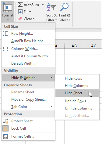
2. On the Home tab, in the Cells group, click Format > Visibility > Hide & Unhide > Hide Sheet.

   

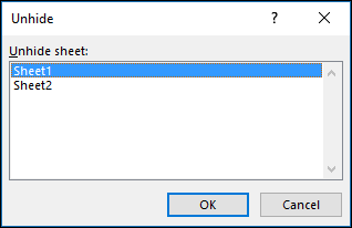
3. To unhide worksheets, follow the same steps, but select Unhide. You’ll be presented with a dialog box listing which sheets are hidden, so select the ones you want to unhide.

   

   Note: Worksheets hidden by VBA code have the property xlSheetVeryHidden; the Unhide command will not display those hidden sheets. If you are using a workbook that contains VBA code and you encounter problems with hidden worksheets, contact the workbook owner for more information.

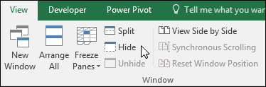
Hide or unhide a workbook window

• On the View tab, in the Window group, click Hide or Unhide.

  On a Mac, this is under the Window menu in the file menu above the ribbon.

  

Notes: 

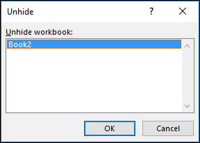
• When you Unhide a workbook, select from the list in the Unhide dialog box.

  

• If Unhide is unavailable, the workbook does not contain hidden workbook windows.

• When you exit Excel, you will be asked if you want to save changes to the hidden workbook window. Click Yes if you want the workbook window to be the same as you left it (hidden or unhidden), the next time that you open the workbook.

Hide or display workbook windows on the Windows taskbar

Excel 2013 introduced the Single Document Interface, where each workbook opens in its own window.

1. Click File > Options.

   For Excel 2007, click the Microsoft Office Button , then Excel Options.

2. Then click Advanced > Display > clear or select the Show all windows in the Taskbar check box.

Hide or unhide a worksheet

1. Select the worksheets that you want to hide.

   How to select worksheets

   To select	Do this
   A single sheet	Click the sheet tab. If you don’t see the tab that you want, click the scrolling buttons to the left of the sheet tabs to display the tab, and then click the tab.
   Two or more adjacent sheets	Click the tab for the first sheet. Then hold down Shift while you click the tab for the last sheet that you want to select.
   Two or more nonadjacent sheets	Click the tab for the first sheet. Then hold down Command while you click the tabs of the other sheets that you want to select.
   All sheets in a workbook	Right-click a sheet tab, and then click Select All Sheets on the shortcut menu.

2. On the Home tab, click Format > under Visibility > Hide & Unhide > Hide Sheet.

3. To unhide worksheets, follow the same steps, but select Unhide. The Unhide dialog box displays a list of hidden sheets, so select the ones you want to unhide and then select OK.

   

Hide or unhide a workbook window

• Click the Window menu, click Hide or Unhide.

Notes: 

• When you Unhide a workbook, select from the list of hidden workbooks in the Unhide dialog box.

  

• If Unhide is unavailable, the workbook does not contain hidden workbook windows.

• When you exit Excel, you will be asked if you want to save changes to the hidden workbook window. Click Yes if you want the workbook window to be the same as you left it (hidden or unhidden) the next time that you open the workbook.

Hide a worksheet

1. Right click on the tab you want to hide.
   

2. Select Hide.

Unhide a worksheet

1. Right click on any visible tab.

2. Select Unhide.
   

3. Mark the tabs to unhide.
   

4. Click OK.

Not sure why you’d have to extract all the sheet names.

Hiding sheets

AFAIK there are two ways to do it.

Select all the sheets that you want to hide, and then right-click and select «hide».
Or, On the Home tab, in the Cells group, click Format,
and under Visibility, click Hide & Unhide, and then click Hide Sheet.

The other way of doing it is by looping the sheets with a simple macro, hiding all sheets apart from the currently selected one:

Sub hideSheets()
Dim wS As Worksheet, Current As String
Current = ActiveSheet.Name
For Each wS In Worksheets
    If Not wS.Name = Current Then
        wS.Visible = False
    End If
Next
End Sub

Showing sheets

To show all the sheets again, the code is even simpler.

Sub showSheets()
Dim wS As Worksheet
For Each wS In Worksheets
        wS.Visible = True
Next
End Sub

Extra

If you want to target a specific sheet, that isn’t the currently active one (to hide all but, or show all but), simply change the Current = ActiveSheet.Name to Current = InputBox("Enter Sheet Name") and you get to name the sheet in an inputbox instead.

If you’re a Microsoft Excel user, it doesn’t take long before you have many different workbooks full of important spreadsheets. What happens when you need to combine these multiple workbooks together so that all of the sheets are in the same place?

Excel can be challenging at times because it’s so powerful. You know that what you want to do is possible, but you might not know how to accomplish it. In this tutorial, I’ll show you several techniques you can use to merge Excel spreadsheets.

When you need to combine multiple spreadsheets, don’t copy and paste the data from each sheet manually. There are many shortcuts that you can use to save time in combining workbooks, and I’ll show you which one is right for each situation.

Watch & Learn

The screencast below will show you how to combine Excel sheets into a single consolidated workbook. I’ll teach you to use PowerQuery (also called Get & Transform Data) to pull together data from multiple workbooks.

Important: The email addresses used in this tutorial are fictitious (randomly generated) and not intended to represent any real email addresses.

Read on to see written instructions. As always, Excel has multiple ways to accomplish this task, and how you’re working with your data will drive which approach is the best.

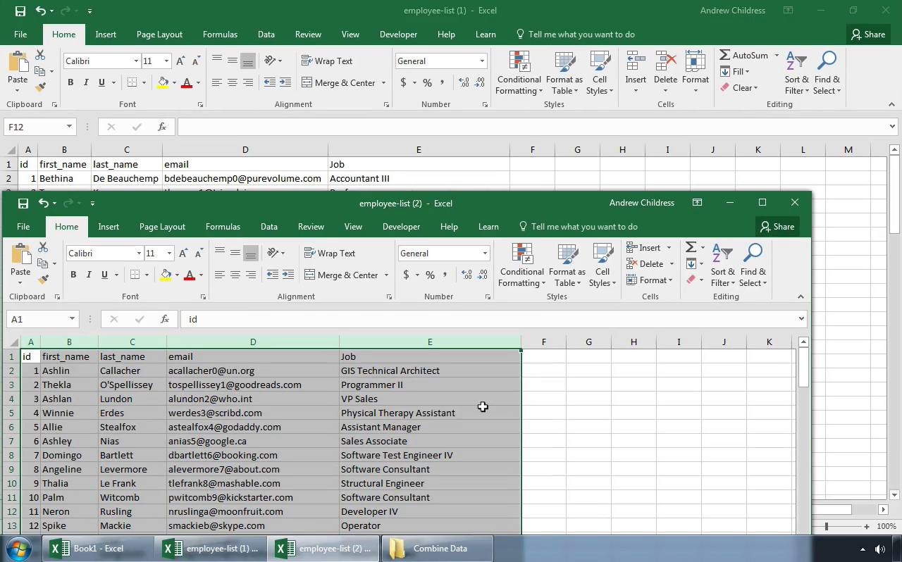
1. How to Move & Copy Sheets (Simplest Method)

The easiest method to merge Excel spreadsheets is to simply take the entire sheet and copy it from one workbook to another.

To do this, start off by opening both Excel workbooks. Then, switch to the workbook that you want to copy several sheets from.

Now, hold Control (or Command on Mac) on your keyboard and click on all of the sheets that you want to copy to a separate workbook. You’ll notice that as you do this, the tabs will show as highlighted.

Now, simply right click and choose Move or Copy from the menu.

On the Move or Copy pop up window, the first thing that you’ll want to do is select the workbook that you want to move the sheets to. Choose the name of the file from the «To book» drop-down.

Also, you can choose where the sheets are placed in the new workbook in terms of sequence. The Before sheet menu controls where sequentially in the workbook the sheets will be inserted. You can always choose (move to end) and re-sequence the order the sheets later as needed.

Finally, it’s optional check the box to Create a copy, which will duplicate the sheets and create a separate copy of them in the workbook you’re moving the sheets to. Once you press OK, you’ll see that the sheets we copied are in the combined workbook.

This approach has a few downsides. If you keep working with two separate files, they aren’t «in sync.» If you make changes to the original workbook that you copied the sheets from, they won’t automatically update in the combined workbook.

2. Prepare to Use Get & Transform Data Tools to Combine Sheets

Excel has an incredibly powerful set of tools that are often called PowerQuery. Beginning with Excel 2016, this feature set was rebranded as Get & Transform Data. 

As the name suggests, these are a set of tools that helps you pull data together from other workbooks and consolidate it into one workbook.

Also, this feature is exclusive to Excel for Windows. You won’t find it in the Mac versions or in the web browser edition of Microsoft’s app.

Before You Start: Check the Data

The most important part of this process is checking your data before you start combining it. The files need to have the same setup for the data structure, with the same columns. You can’t easily combine a four-column spreadsheet and a five-column spreadsheet, as Excel won’t know where to place the data.

Often, you’ll find yourself needing to combine spreadsheets when you’re downloading data from systems. In that case, it’s much easier to make sure the system you’re downloading data is configured to download data in the same columns each time.

Before I download data from a service like Google Analytics, I always make sure that I’m downloading the same report format each time. This ensures that I can easily work with and combine multiple spreadsheets together.

Whether you’re pulling data from a system like Google Analytics, MailChimp, or an ERP like SAP or Oracle that powers huge companies, the best way to save time is to ensure that you’re downloading data in a common format.

Now that we’ve checked our data, it’s time to dive into learning how to combine Excel sheets. 

3. How to Combine Excel Sheets in a Folder Full of Files

A few times, I’ve had a folder full of files that I needed to put together into a single, consolidated file. When you’ve got dozens or even hundreds of files, opening them one-by-one to combine them just isn’t feasible. Learning this technique can save you dozens of hours on a single project.

Again, it’s crucial that the data is in the same format. To get started, it helps to place all of the files in the same folder so that Excel can easily watch this folder for changes. 

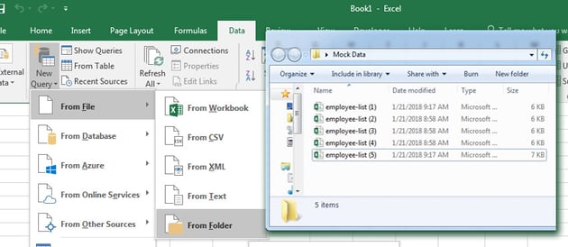
Step 1. Point Excel to the Folder of Files

On the pop-up window, you’ll want to specify a path to the folder that holds your Excel workbooks.

You can browse to that path, or simply paste in the path to the folder with your workbooks.

Step 2. Confirm the List of Files

After you show Excel where the workbooks are stored, a new window will pop up that shows the list of files you’re set to combine. Right now, you’re only seeing metadata about the files, and not the data inside of it.

This window simply shows the files that are going to be combined with our query. You’ll see the file name, the type, and the dates accessed and modified. If you’re missing a file in this list, confirm that all of the files are in the folder and retry the process.

To move on to the next step, click on Edit. 

Step 3. Confirm the Combination

The next menu helps to confirm the data inside your files. Since we’ve already checked that data is the same structure in our multiple files, we can simply click OK on this step.

Step 4. How to Combine Excel Sheets With a Click

Now, a new window pops up with the list of files we’re set to combine.

At this stage, you’re still seeing metadata about the files and now the data itself. To solve that, click on the double drop-down arrow in the upper right corner of the first column.

Voila! Now, you’ll see the actual data from inside the files combined into one place. 

Scroll through the data to confirm that all of your rows are there. Notice that the only change from your original data is that the filename of each source file is in the first column.

Step 5. Close and Load the Data

Believe it or not, we’re basically finished with combining our Excel spreadsheets. The data is in the Query Editor for now, so we’ll need to «send it back» to regular Excel so that we can work with it.

Click on Close & Load in the upper right corner. You’ll see the finished data in a regular Excel spreadsheet, ready to review and work with.

Imagine using this feature to roll up multiple files from different members of your team. Choose a folder that you’ll each store files in, and then combine them into one cohesive file with this feature in just a few minutes.

Recap & Keep Learning

In this tutorial, you learned several techniques for how to combine Excel sheets. When you’ve got many sheets that you need to stitch together, using one of these approaches will save you time so that you can get back to the task at hand!

Check out some of the other tutorials to level up your Excel skills. Each of these tutorials will teach you a method for accomplishing tasks in less time in Microsoft Excel.

How do you merge Excel workbooks? Let me know in the comments section below whether you’ve got a preference for these methods, or a technique of your own that you use.

Did you find this post useful?

I believe that life is too short to do just one thing. In college, I studied Accounting and Finance but continue to scratch my creative itch with my work for Envato Tuts+ and other clients. By day, I enjoy my career in corporate finance, using data and analysis to make decisions.

I cover a variety of topics for Tuts+, including photo editing software like Adobe Lightroom, PowerPoint, Keynote, and more. What I enjoy most is teaching people to use software to solve everyday problems, excel in their career, and complete work efficiently. Feel free to reach out to me on my website.