
Select the cells that you want to display all contents, and click Home > Wrap Text. Then the selected cells will be expanded to show all contents.
Contents
- 1 How do you show all cells?
- 2 Why is Excel not showing cells?
- 3 How do you show hidden cells in Excel?
- 4 How do I get cells to show all text in sheets?
- 5 How do I unhide all rows in Excel?
- 6 How do I view entire Excel spreadsheet?
- 7 Why my Excel open but not visible?
- 8 How do I unhide all columns?
- 9 What is the wrap text?
- 10 How do I make multiple lines in one cell in Google Sheets?
- 11 How do you tag your team on your spreadsheet or DOC file?
- 12 How do I unhide multiple rows at once?
- 13 Can only see Excel sheet in full screen?
- 14 Where is normal view in Excel?
- 15 What is normal view in Excel?
- 16 Can’t Maximise Excel window?
- 17 Why is my Excel File not showing anything?
- 18 Why did my Excel File disappear?
- 19 How do I unhide all rows and columns in Excel?
- 20 How do I expand all columns in Excel?
Press Ctrl + Shift + 9 to unhide all rows or Ctrl + Shift + 0 (zero) to unhide all columns. If this doesn’t work, then right-click on a row or column identifier and select Unhide.
Why is Excel not showing cells?
Your Excel worksheet won’t display data in cells if it is corrupted. In other words, the cell values won’t display any result if the data in your Excel worksheet is damaged or corrupted. In that case, you can manually fix and recover corrupt Excel files or use an Excel repair tool, such as Stellar Repair for Excel.
How do you show hidden cells in Excel?
On the Home tab, in the Cells group, click Format. Do one of the following: Under Visibility, click Hide & Unhide, and then click Unhide Rows or Unhide Columns.
How do I get cells to show all text in sheets?
How to Wrap Text in Google Sheets
- Select the cells you want to set to wrap.
- Click Format.
- Select Text wrapping.
- Select Wrap.
How do I unhide all rows in Excel?
How to unhide all rows in Excel
- To unhide all hidden rows in Excel, navigate to the “Home” tab.
- Click “Format,” which is located towards the right hand side of the toolbar.
- Navigate to the “Visibility” section.
- Hover over “Hide & Unhide.”
- Select “Unhide Rows” from the list.
How do I view entire Excel spreadsheet?
Switch to full or normal screen view in Excel
- To switch to full screen view, on the View tab, in the Workbook Views group, click Full Screen.
- To return to normal screen view, right-click anywhere in the worksheet, and then click Close Full Screen.
Why my Excel open but not visible?
This could be as a result of an intentional or accidental hiding of the workbook (as apposed to a sheet).In order to see it again, click the UNHIDE option in the VIEW tab and it will give you a list of hidden workbooks. You can then choose the one you want to see and click OK, and it will re appear.
How do I unhide all columns?
Here are the steps to unhide all columns at one go:
- Click on the small triangle at the top left of the worksheet area. This will select all the cells in the worksheet.
- Right-click anywhere in the worksheet area.
- Click on Unhide.
What is the wrap text?
“Wrapping text” means displaying the cell contents on multiple lines, rather than one long line. This will allow you to avoid the “truncated column” effect, make the text easier to read and better fit for printing. In addition, it will help you keep the column width consistent throughout the entire worksheet.
How do I make multiple lines in one cell in Google Sheets?
Thankfully, you can – to type information into more than one line in a Google Sheets cell, click on the cell in question and type the first line of your content in. Then, press Alt + Enter on your keyboard (or Option + Enter if you use a Mac) to get to a new line.
How do you tag your team on your spreadsheet or DOC file?
1. Open a new or previously saved Google document. 2. Type “@,” then start typing the name or email address of the person you want to tag.
How do I unhide multiple rows at once?
The skipped number rows are the hidden row. Click the symbol to select the whole sheet. Now Right click anywhere on the mouse to view options. Select Unhide option to unhide all the rows at once.
Can only see Excel sheet in full screen?
The spreadsheet appears if you select Full Screen from the View tab. Open the spreadsheet. On the View tab in the Window section, click Arrange All. In the “Arrange Windows” window, select Tiled and click OK.
Where is normal view in Excel?
Click the top “View” tab and click “Normal” from the Workbook Views group to return to Normal view.
What is normal view in Excel?
The Normal view in Excel 2013 is the one that the program opens to by default. This will display only the cells in your spreadsheet. You will not see the header and footer, nor will you see the page breaks.
Can’t Maximise Excel window?
Try opening the files in safe mode and check the result; * Hold Windows key + R. Note: There is space between Excel and /. If the issue does not occur in Excel safe, then try to disable add-ins associated with Excel and check the result.
Why is my Excel File not showing anything?
Sometimes, when a user opens a saved workbook, it is blank. This issue is often caused when Excel’s settings are changed (usually inadvertently) to ignore external programs.
Why did my Excel File disappear?
If your Excel file disappeared. Sudden power failure can cause your Excel spreadsheet not to be saved and probably disappear from your computer. Also, if Excel is not responding and then it is forced to close, the current spreadsheet being worked on may not be saved.
How do I unhide all rows and columns in Excel?
To unhide all rows and columns, select the whole sheet as explained above, and then press Ctrl + Shift + 9 to show hidden rows and Ctrl + Shift + 0 to show hidden columns.
How do I expand all columns in Excel?
Left-click the mouse button in the header between the columns or rows that you selected and drag the mouse to the left and right for columns and up and down for the rows to adjust the size of all of the selected columns at once. That’s it.
Содержание
- How to show formulas in Excel
- How to show formulas in Excel
- 1. Show Formulas option on the Excel ribbon
- 2. Show formulas in cells instead of their results in Excel options
- 3. Excel shortcut to show formulas
- How to print formulas in Excel
- Why is Excel showing formula, not result?
- 3 Quick Ways to Select Visible Cells in Excel
- Select Visible Cells using a Keyboard Shortcut
- Select Visible Cells using Go To Special Dialog Box
- Select Visible Cells using a QAT Command
- Главные свойства Range и Cells
- Краткое руководство по диапазонам и клеткам
- Введение
- Важное замечание
- Свойство Range
- Свойство Cells рабочего листа
- Использование Cells и Range вместе
- Свойство Offset диапазона
- Использование диапазона CurrentRegion
- Использование Rows и Columns в качестве Ranges
- Использование Range вместо Worksheet
- Чтение значений из одной ячейки в другую
- Использование метода Range.Resize
- Чтение Value в переменные
- Как копировать и вставлять ячейки
- Чтение диапазона ячеек в массив
- Пройти через все клетки в диапазоне
- Форматирование ячеек
- Основные моменты
How to show formulas in Excel
 by Svetlana Cheusheva, updated on February 7, 2023
In this short tutorial, you will learn an easy way to display formulas in Excel 2016, 2013, 2010 and older versions. Also, you will learn how to print formulas and why sometimes Excel shows a formula, not result, in a cell.
If you are working on a spreadsheet with a lot of formulas in it, it may become challenging to comprehend how all those formulas relate to each other. Showing formulas in Excel instead of their results can help you track the data used in each calculation and quickly check your formulas for errors.
Microsoft Excel provides a really simple and quick way to show formulas in cells, and in a moment, you will make sure of this.
How to show formulas in Excel
Usually, when you enter a formula in a cell and press the Enter key, Excel immediately displays the calculated result. To show all formulas in the cells containing them, use one of the following methods.
1. Show Formulas option on the Excel ribbon
In your Excel worksheet, go to the Formulas tab > Formula Auditing group and click the Show Formulas button.
Microsoft Excel displays formulas in cells instead of their results right away. To get the calculated values back, click the Show Formulas button again to toggle it off. 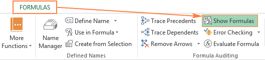
2. Show formulas in cells instead of their results in Excel options
In Excel 2010 and higher, go to File > Options. In Excel 2007, click Office Button > Excel Options.
Select Advanced on the left pane, scroll down to the Display options for this worksheet section and select the option Show formulas in cells instead of their calculated results.
At first sight, this seems to be a longer way, but you may find it useful when you want to display formulas in a number of Excel sheets, within the currently open workbooks. In this case, you just select the sheet name from the dropdown list and check the Show formulas in cells… option for each sheet. 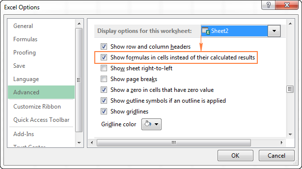
3. Excel shortcut to show formulas
The fastest way to see every formula in your Excel spreadsheet is pressing the following shortcut: Ctrl + `
The grave accent key (`) is the furthest key to the left on the row with the number keys (next to the number 1 key).
The Show Formulas shortcut toggles between displaying cell values and cell formulas. To get the formula results back, simply hit the shortcut again.
Note. Whichever of the above methods you use, Microsoft Excel will show all formulas of the current worksheet. To display formulas in other sheets and workbooks, you will need to repeat the process for each sheet individually.
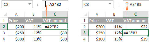
If you want to view the data used in a formula’s calculations, use any of the above methods to show formulas in cells, then select the cell containing the formula in question, and you will see a result similar to this: 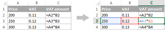
Tip. If you click a cell with a formula, but the formula does not show up in the formula bar, then most likely that formula is hidden and the worksheet is protected. Here are the steps to unhide formulas and remove the worksheet protection.
How to print formulas in Excel
If you want to print formulas in your Excel spreadsheet instead of printing the calculated results of those formulas, just use any of the 3 methods to show formulas in cells, and then print the worksheet as you normally print your Excel files (File > Print). That’s it!
Why is Excel showing formula, not result?
Did it ever happen to you that you type a formula in a cell, press the Enter key… and Excel still shows the formula instead of the result? Don’t worry, your Excel is all right, and we will have that mishap fixed in a moment.
In general, Microsoft Excel can display formulas instead of calculated values for the following reasons:
- You may have inadvertently activated the Show Formulas mode by clicking the corresponding button on the ribbon, or pressing the CTRL+` shortcut. To get the calculated results back, just toggle off the Show Formulas button or press CTRL+` again.
- You may have accidentally typed a space or single quote (‘) before the equal sign in the formula:

When a space or single quote precedes the equal sign, Excel treats the cell contents as text and does not evaluate any formula within that cell. To fix this, just remove the leading space or single quote.
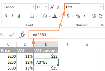
To fix this error, select the cell, go to the Home tab > Number group, and set the cell’s formatting to General, and while in the cell, press F2 and ENTER.
This is how you show formulas in Excel. A piece of cake, isn’t it? On the other hand, if you plan to share your worksheet with other users, you may want to protect your formulas from overwriting or editing, and even hide them from viewing. And it is exactly what we are going to discuss in the next article. Please stay tuned!
Источник
3 Quick Ways to Select Visible Cells in Excel
Watch Video – 3 Ways to Select Visible Cells in Excel
What do you do when you have to copy a range of cells in Excel and paste it somewhere else?
In most cases, the below three steps get the work done:
- Select the cells that you want to copy.
- Copy the cells (Control + C).
- Select the destination cell and paste these cells (Control + V).
But what if you have some hidden cells in the dataset?
Then – these above three steps are not enough.
Let me show you what happens when you try to copy cells that have hidden rows/columns in it.
Suppose you have a dataset as shown below:

Note that there are hidden rows in this dataset (look at the row numbers).
Now see what happens when I try to copy these cells and paste it somewhere else.

In the above example, I selected the visible cells, but when I paste these cells into another location, it copied the visible as well as the hidden cells.
The workaround to this is to make sure that Excel only selects the visible cells. Then I can copy and paste these visible cells only.
In this tutorial, I will show you three ways to select visible cells only in Excel.
This Tutorial Covers:
Select Visible Cells using a Keyboard Shortcut
The easiest way to select visible cells in Excel is by using the following keyboard shortcut:
- For windows: ALT + ; (hold the ALT key and then press the semicolon key)
- For Mac: Cmd+Shift+Z
Here is a screencast where I select only the visible cells, copy the visible cells (notice the marching ants around selection), and paste these:

Select Visible Cells using Go To Special Dialog Box
While using the keyboard shortcut is the fastest way to select visible cells, if you don’t want to use the keyboard or don’t remember the shortcut, there is another way.
You can use the ‘Go To Special’ dialog box to select visible cells in a dataset.
Here are the steps:
- Select the data set in which you want to select the visible cells.
- Go to the Home tab.
- In the Editing group, click on Find and Select.
- Click on Go To Special.
- In the ‘Go To Special’ dialog box, select ‘Visible cells only’.
- Click OK.


This would select all the visible cells in the dataset.
Select Visible Cells using a QAT Command
Another great way to select visible cells in Excel is to add a command to the Quick Access Toolbar (QAT).
Once added, you can simply click this command in the QAT, and it will select visible cells in the dataset.
Here are the steps to add ‘Select Visible Cells’ command to the QAT:
- Click on the Customize Quick Access Toolbar icon.
- Select ‘More Commands’.
- In the ‘Excel Options’ dialogue box, from the ‘Choose command from’ drop-down, select ‘All Commands’.
- Scroll down the list and click on ‘Select Visible Cells’ option.
- Click on the Add button.
- Click OK.


The above steps would add the ‘Select Visible Cells’ command to the QAT.

Now you when you select a dataset and click on this command in the QAT, it will select visible cells only.
You May Also Like the Following Excel Tutorials:
Источник
Главные свойства Range и Cells

Это большая ошибка — теоретизировать, прежде чем кто-то получит данные
Эта статья охватывает все, что вам нужно знать об использовании ячеек и диапазонов в VBA. Вы можете прочитать его от начала до конца, так как он сложен в логическом порядке. Или использовать оглавление ниже, чтобы перейти к разделу по вашему выбору.
Рассматриваемые темы включают свойство смещения, чтение значений между ячейками, чтение значений в массивы и форматирование ячеек.
Краткое руководство по диапазонам и клеткам
| Функция | Принимает | Возвращает | Пример | Вид |
| Range | адреса ячеек |
диапазон ячеек |
.Range(«A1:A4») | $A$1:$A$4 |
| Cells | строка, столбец |
одна ячейка |
.Cells(1,5) | $E$1 |
| Offset | строка, столбец |
диапазон | .Range(«A1:A2») .Offset(1,2) |
$C$2:$C$3 |
| Rows | строка (-и) | одна или несколько строк |
.Rows(4) .Rows(«2:4») |
$4:$4 $2:$4 |
| Columns | столбец (-цы) |
один или несколько столбцов |
.Columns(4) .Columns(«B:D») |
$D:$D $B:$D |
Введение
Это третья статья, посвященная трем основным элементам VBA. Этими тремя элементами являются Workbooks, Worksheets и Ranges/Cells. Cells, безусловно, самая важная часть Excel. Почти все, что вы делаете в Excel, начинается и заканчивается ячейками.
Вы делаете три основных вещи с помощью ячеек:
- Читаете из ячейки.
- Пишите в ячейку.
- Изменяете формат ячейки.
В Excel есть несколько методов для доступа к ячейкам, таких как Range, Cells и Offset. Можно запутаться, так как эти функции делают похожие операции.
В этой статье я расскажу о каждом из них, объясню, почему они вам нужны, и когда вам следует их использовать.
Давайте начнем с самого простого метода доступа к ячейкам — с помощью свойства Range рабочего листа.
Важное замечание
Я недавно обновил эту статью, сейчас использую Value2.
Вам может быть интересно, в чем разница между Value, Value2 и значением по умолчанию:
Использование Value может усечь число, если ячейка отформатирована, как валюта. Если вы не используете какое-либо свойство, по умолчанию используется Value.
Лучше использовать Value2, поскольку он всегда будет возвращать фактическое значение ячейки.
Свойство Range
Рабочий лист имеет свойство Range, которое можно использовать для доступа к ячейкам в VBA. Свойство Range принимает тот же аргумент, что и большинство функций Excel Worksheet, например: «А1», «А3: С6» и т.д.
В следующем примере показано, как поместить значение в ячейку с помощью свойства Range.
Как видно из кода, Range является членом Worksheets, которая, в свою очередь, является членом Workbook. Иерархия такая же, как и в Excel, поэтому должно быть легко понять. Чтобы сделать что-то с Range, вы должны сначала указать рабочую книгу и рабочий лист, которому она принадлежит.
В оставшейся части этой статьи я буду использовать кодовое имя для ссылки на лист.

Следующий код показывает приведенный выше пример с использованием кодового имени рабочего листа, т.е. Лист1 вместо ThisWorkbook.Worksheets («Лист1»).
Вы также можете писать в несколько ячеек, используя свойство Range
Свойство Cells рабочего листа
У Объекта листа есть другое свойство, называемое Cells, которое очень похоже на Range . Есть два отличия:
- Cells возвращают диапазон только одной ячейки.
- Cells принимает строку и столбец в качестве аргументов.
В приведенном ниже примере показано, как записывать значения в ячейки, используя свойства Range и Cells.
Вам должно быть интересно, когда использовать Cells, а когда Range. Использование Range полезно для доступа к одним и тем же ячейкам при каждом запуске макроса.
Например, если вы использовали макрос для вычисления суммы и каждый раз записывали ее в ячейку A10, тогда Range подойдет для этой задачи.
Использование свойства Cells полезно, если вы обращаетесь к ячейке по номеру, который может отличаться. Проще объяснить это на примере.
В следующем коде мы просим пользователя указать номер столбца. Использование Cells дает нам возможность использовать переменное число для столбца.
В приведенном выше примере мы используем номер для столбца, а не букву.
Чтобы использовать Range здесь, потребуется преобразовать эти значения в ссылку на буквенно-цифровую ячейку, например, «С1». Использование свойства Cells позволяет нам предоставить строку и номер столбца для доступа к ячейке.
Иногда вам может понадобиться вернуть более одной ячейки, используя номера строк и столбцов. В следующем разделе показано, как это сделать.
Использование Cells и Range вместе
Как вы уже видели, вы можете получить доступ только к одной ячейке, используя свойство Cells. Если вы хотите вернуть диапазон ячеек, вы можете использовать Cells с Range следующим образом:
Как видите, вы предоставляете начальную и конечную ячейку диапазона. Иногда бывает сложно увидеть, с каким диапазоном вы имеете дело, когда значением являются все числа. Range имеет свойство Address, которое отображает буквенно-цифровую ячейку для любого диапазона. Это может пригодиться, когда вы впервые отлаживаете или пишете код.
В следующем примере мы распечатываем адрес используемых нами диапазонов.
В примере я использовал Debug.Print для печати в Immediate Window. Для просмотра этого окна выберите «View» -> «в Immediate Window» (Ctrl + G).


Свойство Offset диапазона
У диапазона есть свойство, которое называется Offset. Термин «Offset» относится к отсчету от исходной позиции. Он часто используется в определенных областях программирования. С помощью свойства «Offset» вы можете получить диапазон ячеек того же размера и на определенном расстоянии от текущего диапазона. Это полезно, потому что иногда вы можете выбрать диапазон на основе определенного условия. Например, на скриншоте ниже есть столбец для каждого дня недели. Учитывая номер дня (т.е. понедельник = 1, вторник = 2 и т.д.). Нам нужно записать значение в правильный столбец.

Сначала мы попытаемся сделать это без использования Offset.
Как видно из примера, нам нужно добавить строку для каждого возможного варианта. Это не идеальная ситуация. Использование свойства Offset обеспечивает более чистое решение.
Как видите, это решение намного лучше. Если количество дней увеличилось, нам больше не нужно добавлять код. Чтобы Offset был полезен, должна быть какая-то связь между позициями ячеек. Если столбцы Day в приведенном выше примере были случайными, мы не могли бы использовать Offset. Мы должны были бы использовать первое решение.
Следует иметь в виду, что Offset сохраняет размер диапазона. Итак .Range («A1:A3»).Offset (1,1) возвращает диапазон B2:B4. Ниже приведены еще несколько примеров использования Offset.
Использование диапазона CurrentRegion
CurrentRegion возвращает диапазон всех соседних ячеек в данный диапазон. На скриншоте ниже вы можете увидеть два CurrentRegion. Я добавил границы, чтобы прояснить CurrentRegion.

Строка или столбец пустых ячеек означает конец CurrentRegion.
Вы можете вручную проверить CurrentRegion в Excel, выбрав диапазон и нажав Ctrl + Shift + *.
Если мы возьмем любой диапазон ячеек в пределах границы и применим CurrentRegion, мы вернем диапазон ячеек во всей области.
Range («B3»). CurrentRegion вернет диапазон B3:D14
Range («D14»). CurrentRegion вернет диапазон B3:D14
Range («C8:C9»). CurrentRegion вернет диапазон B3:D14 и так далее
Как пользоваться
Мы получаем CurrentRegion следующим образом
Только чтение строк данных
Прочитать диапазон из второй строки, т.е. пропустить строку заголовка.
Удалить заголовок
Удалить строку заголовка (т.е. первую строку) из диапазона. Например, если диапазон — A1:D4, это возвратит A2:D4
Использование Rows и Columns в качестве Ranges
Если вы хотите что-то сделать со всей строкой или столбцом, вы можете использовать свойство «Rows и Columns» на рабочем листе. Они оба принимают один параметр — номер строки или столбца, к которому вы хотите получить доступ.
Использование Range вместо Worksheet
Вы также можете использовать Cella, Rows и Columns, как часть Range, а не как часть Worksheet. У вас может быть особая необходимость в этом, но в противном случае я бы избегал практики. Это делает код более сложным. Простой код — твой друг. Это уменьшает вероятность ошибок.
Код ниже выделит второй столбец диапазона полужирным. Поскольку диапазон имеет только две строки, весь столбец считается B1:B2
Чтение значений из одной ячейки в другую
В большинстве примеров мы записали значения в ячейку. Мы делаем это, помещая диапазон слева от знака равенства и значение для размещения в ячейке справа. Для записи данных из одной ячейки в другую мы делаем то же самое. Диапазон назначения идет слева, а диапазон источника — справа.
В следующем примере показано, как это сделать:
Как видно из этого примера, невозможно читать из нескольких ячеек. Если вы хотите сделать это, вы можете использовать функцию копирования Range с параметром Destination.
Функция Copy копирует все, включая формат ячеек. Это тот же результат, что и ручное копирование и вставка выделения. Подробнее об этом вы можете узнать в разделе «Копирование и вставка ячеек»
Использование метода Range.Resize
При копировании из одного диапазона в другой с использованием присваивания (т.е. знака равенства) диапазон назначения должен быть того же размера, что и исходный диапазон.
Использование функции Resize позволяет изменить размер диапазона до заданного количества строк и столбцов.
Когда мы хотим изменить наш целевой диапазон, мы можем просто использовать исходный размер диапазона.
Другими словами, мы используем количество строк и столбцов исходного диапазона в качестве параметров для изменения размера:
Мы можем сделать изменение размера в одну строку, если нужно:
Чтение Value в переменные
Мы рассмотрели, как читать из одной клетки в другую. Вы также можете читать из ячейки в переменную. Переменная используется для хранения значений во время работы макроса. Обычно вы делаете это, когда хотите манипулировать данными перед тем, как их записать. Ниже приведен простой пример использования переменной. Как видите, значение элемента справа от равенства записывается в элементе слева от равенства.
Для чтения текста в переменную вы используете переменную типа String.
Вы можете записать переменную в диапазон ячеек. Вы просто указываете диапазон слева, и значение будет записано во все ячейки диапазона.
Вы не можете читать из нескольких ячеек в переменную. Однако вы можете читать массив, который представляет собой набор переменных. Мы рассмотрим это в следующем разделе.
Как копировать и вставлять ячейки
Если вы хотите скопировать и вставить диапазон ячеек, вам не нужно выбирать их. Это распространенная ошибка, допущенная новыми пользователями VBA.
Вы можете просто скопировать ряд ячеек, как здесь:
При использовании этого метода копируется все — значения, форматы, формулы и так далее. Если вы хотите скопировать отдельные элементы, вы можете использовать свойство PasteSpecial диапазона.
В следующей таблице приведен полный список всех типов вставок.
| Виды вставок |
| xlPasteAll |
| xlPasteAllExceptBorders |
| xlPasteAllMergingConditionalFormats |
| xlPasteAllUsingSourceTheme |
| xlPasteColumnWidths |
| xlPasteComments |
| xlPasteFormats |
| xlPasteFormulas |
| xlPasteFormulasAndNumberFormats |
| xlPasteValidation |
| xlPasteValues |
| xlPasteValuesAndNumberFormats |
Чтение диапазона ячеек в массив
Вы также можете скопировать значения, присвоив значение одного диапазона другому.
Значение диапазона в этом примере считается вариантом массива. Это означает, что вы можете легко читать из диапазона ячеек в массив. Вы также можете писать из массива в диапазон ячеек. Если вы не знакомы с массивами, вы можете проверить их в этой статье.
В следующем коде показан пример использования массива с диапазоном.
Имейте в виду, что массив, созданный для чтения, является двумерным массивом. Это связано с тем, что электронная таблица хранит значения в двух измерениях, то есть в строках и столбцах.
Пройти через все клетки в диапазоне
Иногда вам нужно просмотреть каждую ячейку, чтобы проверить значение.
Вы можете сделать это, используя цикл For Each, показанный в следующем коде.
Вы также можете проходить последовательные ячейки, используя свойство Cells и стандартный цикл For.
Стандартный цикл более гибок в отношении используемого вами порядка, но он медленнее, чем цикл For Each.
Форматирование ячеек
Иногда вам нужно будет отформатировать ячейки в электронной таблице. Это на самом деле очень просто. В следующем примере показаны различные форматы, которые можно добавить в любой диапазон ячеек.
Основные моменты
Ниже приводится краткое изложение основных моментов
- Range возвращает диапазон ячеек
- Cells возвращают только одну клетку
- Вы можете читать из одной ячейки в другую
- Вы можете читать из диапазона ячеек в другой диапазон ячеек.
- Вы можете читать значения из ячеек в переменные и наоборот.
- Вы можете читать значения из диапазонов в массивы и наоборот
- Вы можете использовать цикл For Each или For, чтобы проходить через каждую ячейку в диапазоне.
- Свойства Rows и Columns позволяют вам получить доступ к диапазону ячеек этих типов
Источник
Excel for Microsoft 365 Excel 2021 Excel 2019 Excel 2016 Excel 2013 Excel 2010 Excel 2007 More…Less
To select all cells on a worksheet, use one of the following methods:
-
Click the Select All button.
-
Press CTRL+A.
Note If the worksheet contains data, and the active cell is above or to the right of the data, pressing CTRL+A selects the current region. Pressing CTRL+A a second time selects the entire worksheet.

Tip If you want to select all cells in the active range, press CTRL+SHIFT+*.
Need more help?
Want more options?
Explore subscription benefits, browse training courses, learn how to secure your device, and more.
Communities help you ask and answer questions, give feedback, and hear from experts with rich knowledge.
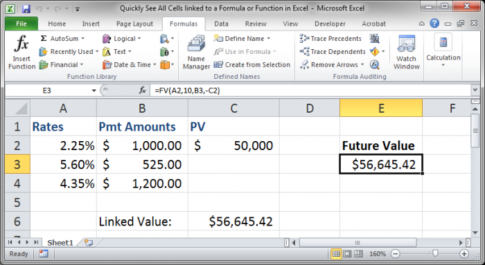
Ill show you how to see the cells used in a formula/function in Excel and also how to tell which cells are using that particular formula/function.
This is a simple yet very helpful feature in Excel and it allows you to visually represent the relationship between the cells/formulas/functions in the worksheet.
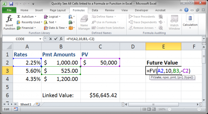
This is actually very easy to do, just select the formula/function for which you want to see the cells it uses or references, and then go to the Formulas tab and click the Trace Precedents button:
Formulas tab > Trace Precedents
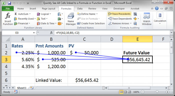
The best part about this feature is that you can now select other cells and go about your work in this worksheet while keeping these arrows visible. This is what makes this different than just double-clicking a formula/function, which also shows the cells used in it.
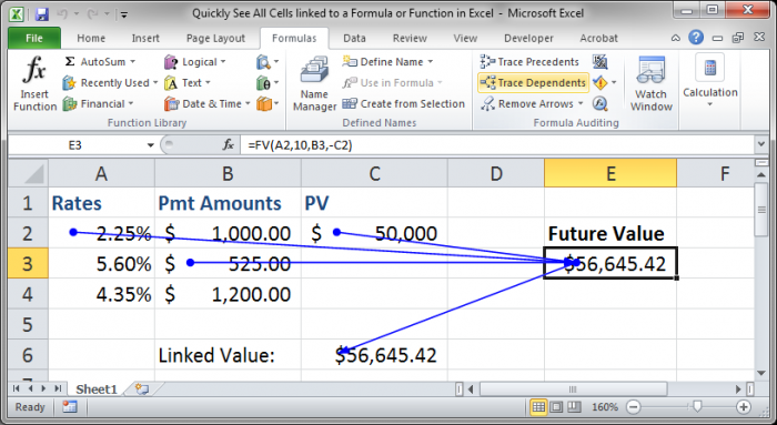
Now, if you wanted to see if there were any cells that referenced this cell/function/formula, simply select it and then click the Trace Dependents button on the Formulas Tab.
Formulas Tab > Trace Dependents
If you want to remove these arrows, simply click the Remove Arrows button or click the arrow next to that button and select which arrows you would like to remove, either the precedent or the dependent ones.
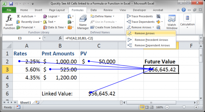
Now we are back where we started.
Remember that if you just want a quick view of the cells that are used in a formula or function you just have to double-click the desired cell and you will see a nice representation of the precedent cells in the worksheet.
However, this representation of the precedent cells will not stay visible once you have deselected the cell or continued working in the worksheet, and this is why the Trace Precedents and Trace Dependents feature is so useful.
I hope this tutorial was helpful! 
Similar Content on TeachExcel
Guide to Referencing Other Excel Files with Formulas and Functions
Tutorial: Your guide to making cross-workbook formulas and functions. This includes an overview of p…
How to Find and Fix Errors in Complex Formulas in Excel
Tutorial:
Here, I’ll show you a quick, simple, and effective way to fix formulas and functions in E…
Naming Cells in Excel to Make Using Formulas/Functions Easier
Tutorial: In this tutorial I am going to introduce the idea of Named Cells. A Named Cell is a cell w…
Understanding Formulas and Functions in Excel
Tutorial: In this tutorial I will cover the basic concepts of Formulas and Functions in Excel.
A for…
Logical Comparison Operators in Excel — How to Compare Things
Tutorial:
(Video tutorial’s page: Compare Values in Excel — Beginner to Advanced)
Logical compariso…
Subscribe for Weekly Tutorials
BONUS: subscribe now to download our Top Tutorials Ebook!
Watch Video – 3 Ways to Select Visible Cells in Excel
What do you do when you have to copy a range of cells in Excel and paste it somewhere else?
In most cases, the below three steps get the work done:
- Select the cells that you want to copy.
- Copy the cells (Control + C).
- Select the destination cell and paste these cells (Control + V).
But what if you have some hidden cells in the dataset?
Then – these above three steps are not enough.
Let me show you what happens when you try to copy cells that have hidden rows/columns in it.
Suppose you have a dataset as shown below:
Note that there are hidden rows in this dataset (look at the row numbers).
Now see what happens when I try to copy these cells and paste it somewhere else.
In the above example, I selected the visible cells, but when I paste these cells into another location, it copied the visible as well as the hidden cells.
The workaround to this is to make sure that Excel only selects the visible cells. Then I can copy and paste these visible cells only.
In this tutorial, I will show you three ways to select visible cells only in Excel.
Select Visible Cells using a Keyboard Shortcut
The easiest way to select visible cells in Excel is by using the following keyboard shortcut:
- For windows: ALT + ; (hold the ALT key and then press the semicolon key)
- For Mac: Cmd+Shift+Z
Here is a screencast where I select only the visible cells, copy the visible cells (notice the marching ants around selection), and paste these:
Select Visible Cells using Go To Special Dialog Box
While using the keyboard shortcut is the fastest way to select visible cells, if you don’t want to use the keyboard or don’t remember the shortcut, there is another way.
You can use the ‘Go To Special’ dialog box to select visible cells in a dataset.
Here are the steps:
- Select the data set in which you want to select the visible cells.
- Go to the Home tab.

- In the Editing group, click on Find and Select.

- Click on Go To Special.

- In the ‘Go To Special’ dialog box, select ‘Visible cells only’.

- Click OK.
This would select all the visible cells in the dataset.
Also read: Select Till End of Data in a Column in Excel (Shortcuts)
Select Visible Cells using a QAT Command
Another great way to select visible cells in Excel is to add a command to the Quick Access Toolbar (QAT).
Once added, you can simply click this command in the QAT, and it will select visible cells in the dataset.
Here are the steps to add ‘Select Visible Cells’ command to the QAT:
- Click on the Customize Quick Access Toolbar icon.

- Select ‘More Commands’.

- In the ‘Excel Options’ dialogue box, from the ‘Choose command from’ drop-down, select ‘All Commands’.

- Scroll down the list and click on ‘Select Visible Cells’ option.

- Click on the Add button.
- Click OK.
The above steps would add the ‘Select Visible Cells’ command to the QAT.
Now you when you select a dataset and click on this command in the QAT, it will select visible cells only.
You May Also Like the Following Excel Tutorials:
- How to Deselect Cells in Excel
- How to Select Non-adjacent cells in Excel?
- Number Rows in Excel
- How to Hide a Worksheet in Excel (that can’t be unhidden).
- How to Select Every Third Row in Excel (or select every Nth Row).
- Highlight EVERY Other ROW in Excel (using Conditional Formatting).
- How to Quickly Select Blank Cells in Excel.