
Excel for Microsoft 365 Excel 2021 Excel 2019 Excel 2016 Excel 2013 Excel 2010 Excel 2007 More…Less
In Excel, formatting worksheet (or sheet) data is easier than ever. You can use several fast and simple ways to create professional-looking worksheets that display your data effectively. For example, you can use document themes for a uniform look throughout all of your Excel spreadsheets, styles to apply predefined formats, and other manual formatting features to highlight important data.
A document theme is a predefined set of colors, fonts, and effects (such as line styles and fill effects) that will be available when you format your worksheet data or other items, such as tables, PivotTables, or charts. For a uniform and professional look, a document theme can be applied to all of your Excel workbooks and other Office release documents.
Your company may provide a corporate document theme that you can use, or you can choose from a variety of predefined document themes that are available in Excel. If needed, you can also create your own document theme by changing any or all of the theme colors, fonts, or effects that a document theme is based on.
Before you format the data on your worksheet, you may want to apply the document theme that you want to use, so that the formatting that you apply to your worksheet data can use the colors, fonts, and effects that are determined by that document theme.
For information on how to work with document themes, see Apply or customize a document theme.
A style is a predefined, often theme-based format that you can apply to change the look of data, tables, charts, PivotTables, shapes, or diagrams. If predefined styles don’t meet your needs, you can customize a style. For charts, you can customize a chart style and save it as a chart template that you can use again.
Depending on the data that you want to format, you can use the following styles in Excel:
-
Cell styles To apply several formats in one step, and to ensure that cells have consistent formatting, you can use a cell style. A cell style is a defined set of formatting characteristics, such as fonts and font sizes, number formats, cell borders, and cell shading. To prevent anyone from making changes to specific cells, you can also use a cell style that locks cells.
Excel has several predefined cell styles that you can apply. If needed, you can modify a predefined cell style to create a custom cell style.
Some cell styles are based on the document theme that is applied to the entire workbook. When you switch to another document theme, these cell styles are updated to match the new document theme.
For information on how to work with cell styles, see Apply, create, or remove a cell style.
-
Table styles To quickly add designer-quality, professional formatting to an Excel table, you can apply a predefined or custom table style. When you choose one of the predefined alternate-row styles, Excel maintains the alternating row pattern when you filter, hide, or rearrange rows.
For information on how to work with table styles, see Format an Excel table.
-
PivotTable styles To format a PivotTable, you can quickly apply a predefined or custom PivotTable style. Just like with Excel tables, you can choose a predefined alternate-row style that retains the alternate row pattern when you filter, hide, or rearrange rows.
For information on how to work with PivotTable styles, see Design the layout and format of a PivotTable report.
-
Chart styles You apply a predefined style to your chart. Excel provides a variety of useful predefined chart styles that you can choose from, and you can customize a style further if needed by manually changing the style of individual chart elements. You cannot save a custom chart style, but you can save the entire chart as a chart template that you can use to create a similar chart.
For information on how to work with chart styles, see Change the layout or style of a chart.
To make specific data (such as text or numbers) stand out, you can format the data manually. Manual formatting is not based on the document theme of your workbook unless you choose a theme font or use theme colors — manual formatting stays the same when you change the document theme. You can manually format all of the data in a cell or range at the same time, but you can also use this method to format individual characters.
For information on how to format data manually, see Format text in cells.
To distinguish between different types of information on a worksheet and to make a worksheet easier to scan, you can add borders around cells or ranges. For enhanced visibility and to draw attention to specific data, you can also shade the cells with a solid background color or a specific color pattern.
If you want to add a colorful background to all of your worksheet data, you can also use a picture as a sheet background. However, a sheet background cannot be printed — a background only enhances the onscreen display of your worksheet.
For information on how to use borders and colors, see:
Apply or remove cell borders on a worksheet
Apply or remove cell shading
Add or remove a sheet background
For the optimal display of the data on your worksheet, you may want to reposition the text within a cell. You can change the alignment of the cell contents, use indentation for better spacing, or display the data at a different angle by rotating it.
Rotating data is especially useful when column headings are wider than the data in the column. Instead of creating unnecessarily wide columns or abbreviated labels, you can rotate the column heading text.
For information on how to change the alignment or orientation of data, see Reposition the data in a cell.
If you have already formatted some cells on a worksheet the way that you want, there are several ways to copy just those formats to other cells or ranges.
Clipboard commands
-
Home > Paste > Paste Special > Paste Formatting.
-
Home > Format Painter
 .
.
Right click command

-
Point your mouse at the edge of selected cells until the pointer changes to a crosshair.
-
Right click and hold, drag the selection to a range, and then release.
-
Select Copy Here as Formats Only.
Tip If you’re using a single-button mouse or trackpad on a Mac, use Control+Click instead of right click.
Range Extension
Data range formats are automatically extended to additional rows when you enter rows at the end of a data range that you have already formatted, and the formats appear in at least three of five preceding rows. The option to extend data range formats and formulas is on by default, but you can turn it on or off by:
-
Newer versions Selecting File > Options > Advanced > Extend date range and formulas (under Editing options).
-
Excel 2007 Selecting Microsoft Office Button
> Excel Options > Advanced > Extend date range and formulas (under Editing options)).
Need more help?
Want more options?
Explore subscription benefits, browse training courses, learn how to secure your device, and more.
Communities help you ask and answer questions, give feedback, and hear from experts with rich knowledge.
Содержание
- Ways to format a worksheet
- Excel Formatting
- Formatting
- Styling Commands in Ribbon
- Styling Commands, Right Clicking Cells
- Chapter summary
- Apply Conditional Formatting – Multiple Sheets in Excel & Google Sheets
- Apply Conditional Formatting to Multiple Sheets
- Copy-Paste
- Format Painter
- Create a Macro to Apply Conditional Formatting Rule
- Apply Conditional Formatting to Multiple Sheets in Google Sheets
- Copy Conditional Formatting From One Cell
- Copy-Paste
- Paint Format
Ways to format a worksheet
In Excel, formatting worksheet (or sheet) data is easier than ever. You can use several fast and simple ways to create professional-looking worksheets that display your data effectively. For example, you can use document themes for a uniform look throughout all of your Excel spreadsheets, styles to apply predefined formats, and other manual formatting features to highlight important data.
A document theme is a predefined set of colors, fonts, and effects (such as line styles and fill effects) that will be available when you format your worksheet data or other items, such as tables, PivotTables, or charts. For a uniform and professional look, a document theme can be applied to all of your Excel workbooks and other Office release documents.
Your company may provide a corporate document theme that you can use, or you can choose from a variety of predefined document themes that are available in Excel. If needed, you can also create your own document theme by changing any or all of the theme colors, fonts, or effects that a document theme is based on.
Before you format the data on your worksheet, you may want to apply the document theme that you want to use, so that the formatting that you apply to your worksheet data can use the colors, fonts, and effects that are determined by that document theme.
For information on how to work with document themes, see Apply or customize a document theme.
A style is a predefined, often theme-based format that you can apply to change the look of data, tables, charts, PivotTables, shapes, or diagrams. If predefined styles don’t meet your needs, you can customize a style. For charts, you can customize a chart style and save it as a chart template that you can use again.
Depending on the data that you want to format, you can use the following styles in Excel:
Cell styles To apply several formats in one step, and to ensure that cells have consistent formatting, you can use a cell style. A cell style is a defined set of formatting characteristics, such as fonts and font sizes, number formats, cell borders, and cell shading. To prevent anyone from making changes to specific cells, you can also use a cell style that locks cells.
Excel has several predefined cell styles that you can apply. If needed, you can modify a predefined cell style to create a custom cell style.
Some cell styles are based on the document theme that is applied to the entire workbook. When you switch to another document theme, these cell styles are updated to match the new document theme.
For information on how to work with cell styles, see Apply, create, or remove a cell style.
Table styles To quickly add designer-quality, professional formatting to an Excel table, you can apply a predefined or custom table style. When you choose one of the predefined alternate-row styles, Excel maintains the alternating row pattern when you filter, hide, or rearrange rows.
For information on how to work with table styles, see Format an Excel table.
PivotTable styles To format a PivotTable, you can quickly apply a predefined or custom PivotTable style. Just like with Excel tables, you can choose a predefined alternate-row style that retains the alternate row pattern when you filter, hide, or rearrange rows.
For information on how to work with PivotTable styles, see Design the layout and format of a PivotTable report.
Chart styles You apply a predefined style to your chart. Excel provides a variety of useful predefined chart styles that you can choose from, and you can customize a style further if needed by manually changing the style of individual chart elements. You cannot save a custom chart style, but you can save the entire chart as a chart template that you can use to create a similar chart.
For information on how to work with chart styles, see Change the layout or style of a chart.
To make specific data (such as text or numbers) stand out, you can format the data manually. Manual formatting is not based on the document theme of your workbook unless you choose a theme font or use theme colors — manual formatting stays the same when you change the document theme. You can manually format all of the data in a cell or range at the same time, but you can also use this method to format individual characters.
For information on how to format data manually, see Format text in cells.
To distinguish between different types of information on a worksheet and to make a worksheet easier to scan, you can add borders around cells or ranges. For enhanced visibility and to draw attention to specific data, you can also shade the cells with a solid background color or a specific color pattern.
If you want to add a colorful background to all of your worksheet data, you can also use a picture as a sheet background. However, a sheet background cannot be printed — a background only enhances the onscreen display of your worksheet.
For information on how to use borders and colors, see:
For the optimal display of the data on your worksheet, you may want to reposition the text within a cell. You can change the alignment of the cell contents, use indentation for better spacing, or display the data at a different angle by rotating it.
Rotating data is especially useful when column headings are wider than the data in the column. Instead of creating unnecessarily wide columns or abbreviated labels, you can rotate the column heading text.
For information on how to change the alignment or orientation of data, see Reposition the data in a cell.
If you have already formatted some cells on a worksheet the way that you want, there are several ways to copy just those formats to other cells or ranges.
Home > Paste > Paste Special > Paste Formatting.
Home > Format Painter  .
.
Right click command
Point your mouse at the edge of selected cells until the pointer changes to a crosshair.
Right click and hold, drag the selection to a range, and then release.
Select Copy Here as Formats Only.
Tip If you’re using a single-button mouse or trackpad on a Mac, use Control+Click instead of right click.
Data range formats are automatically extended to additional rows when you enter rows at the end of a data range that you have already formatted, and the formats appear in at least three of five preceding rows. The option to extend data range formats and formulas is on by default, but you can turn it on or off by:
Newer versions Selecting File > Options > Advanced > Extend date range and formulas (under Editing options).
Excel 2007 Selecting Microsoft Office Button  > Excel Options > Advanced > Extend date range and formulas (under Editing options)).
Источник
Excel Formatting
Formatting
Excel has many ways to format and style a spreadsheet.
Why format and style your spreadsheet?
- Make it easier to read and understand
- Make it more delicate
Styling is about changing the looks of cells, such as changing colors, font, font sizes, borders, number formats, and so on.
The most used styling functions are:
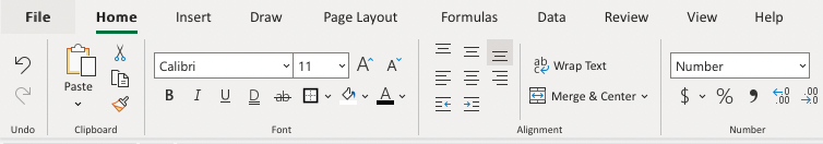
There are two ways to access the styling commands in Excel:
- The Ribbon
- Formatting menu, by right clicking cells
Read more about the Ribbon in the Excel overview chapter.
Styling Commands in Ribbon

The Ribbon can be expanded by clicking the arrow/caret-down icon on the right side. This gives access to more commands:

Styling Commands, Right Clicking Cells
You can also right-click on any cell to style it:
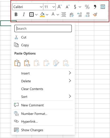
Styling commands can be accessed from both views.
Chapter summary
Formatting is used to make spreadsheets more readable. There are many ways to add styles. The most common ones are; Color, Font, Number format and Grids.
Источник
Apply Conditional Formatting – Multiple Sheets in Excel & Google Sheets
This tutorial demonstrates how to apply conditional formatting to multiple sheets in Excel and Google Sheets.
In the latest versions of Excel, you can no longer select multiple sheets and then apply a conditional formatting rule to all the sheets at once. You need to do one sheet first, then copy the conditional formatting between sheets. Or, you can write a macro to repeat the conditional formatting on each sheet.
Apply Conditional Formatting to Multiple Sheets
Copy-Paste
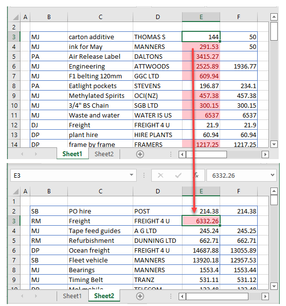
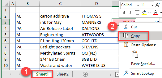
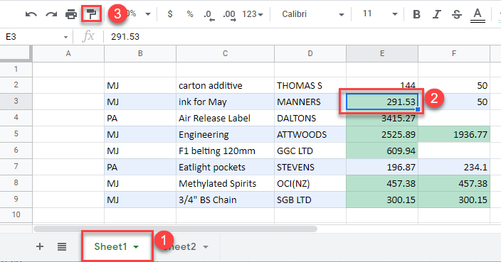
- Select the sheet with the conditional formatting applied and right-click the cell with conditional formatting rule. Then click Copy (or use the keyboard shortcut CTRL + C).
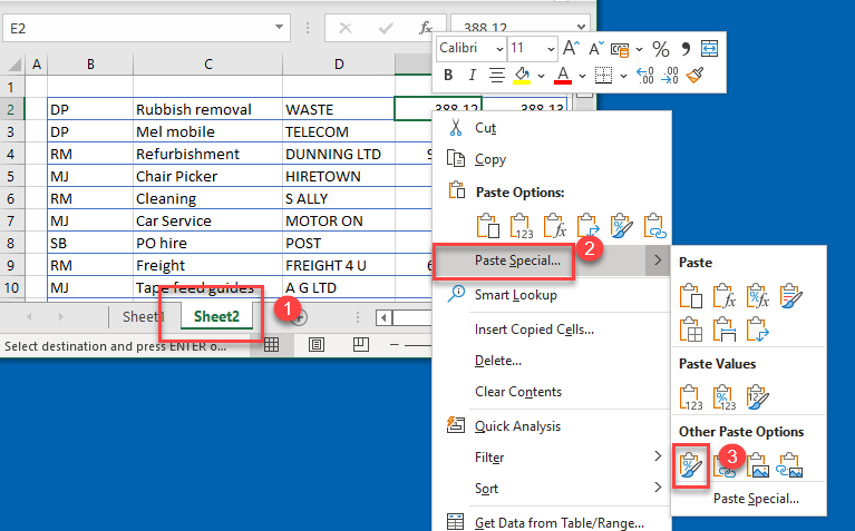
- Next, click on the destination sheet and select the destination cell or cells. Right-click and choose Paste Special > Paste Format.
Format Painter
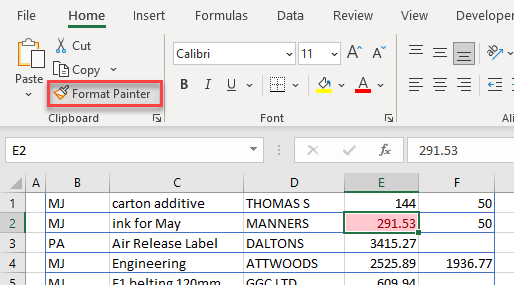
You can also copy the conditional formatting rule from one sheet to another with the Format Painter feature.
- Select the cell in the source sheet that has a conditional formatting rule and then, in the Ribbon, select Home > Clipboard > Format Painter.
- Click on the destination sheet and click on the cells or cell where you wish to apply the format.
Create a Macro to Apply Conditional Formatting Rule
While creating a new conditional formatting rule in Excel, you can record a macro to mimic the steps you take.
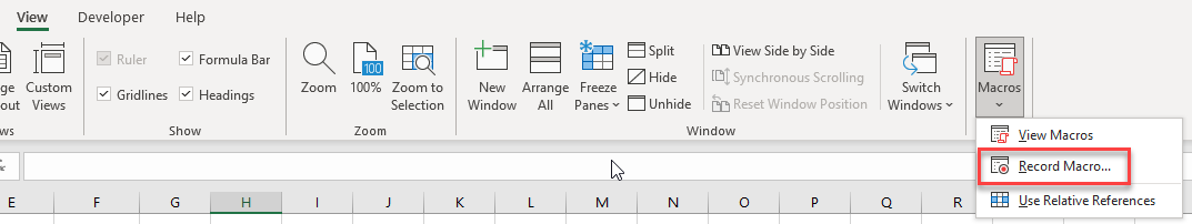
- In the Ribbon, select View > Macros > Record Macro.
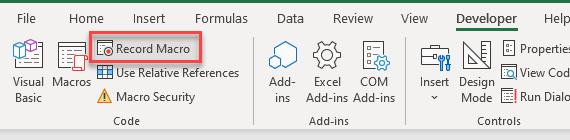
OR, in the Ribbon, select Developer > Code > Record Macro.
Note: If you don’t see the Developer Ribbon, you’ll need to enable it.
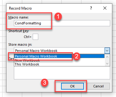
- In the Record Macro dialog box, (1) type in a name for your macro and (2) make sure you select Personal Macro Workbookfrom the drop-down list. Then, (3) click OK to start recording.
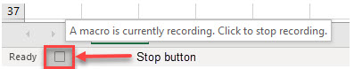
- Once you have clicked OK, you can follow the steps to create the conditional formatting rule you require, and then click the stop button at the bottom of the screen to stop recording the macro.
- To run the macro on a different sheet, switch to that sheet and select the cell or cells you wish to apply the conditional formatting to.
- In the Ribbon, select View > Macros > View Macros.
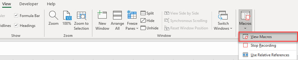
OR Developer > Visual Basic > Macros
- Click on the Macro in the Macro name list and then select Run.
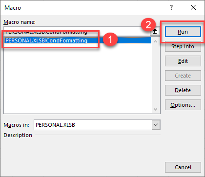
- You can run the macro on as many sheets as you require.
Note: You can view the code by selecting the macro in the Macro dialog box (shown above) and selecting Edit. This takes you to the Visual Basic Editor and enables you to view and/or edit your VBA code.
Apply Conditional Formatting to Multiple Sheets in Google Sheets
You can apply conditional formatting to multiple sheets in Google Sheets in the same way as you do in Excel.
Copy Conditional Formatting From One Cell
Copy-Paste
If you already have a cell or column with a Conditional Formatting rule set up, you can use Copy-Paste to copy the rule to another sheet.
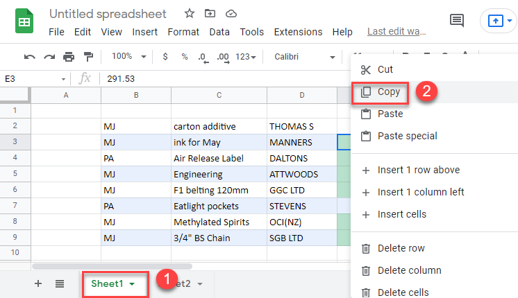
- Right-click on a cell that has the conditional formatting rule applied to it and click Copy (or use the keyboard shortcut CTRL + C).
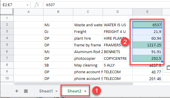
- Select the sheet you require and then select the cell or cells in that sheet where you wish to apply the conditional formatting rule. Select Paste special > Format only (or use the keyboard shortcut CTRL + ALT + V).
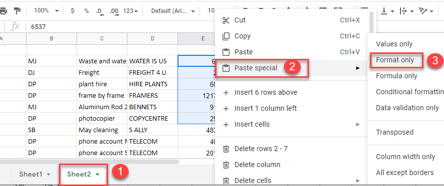
The conditional formatting rule will then be applied to the entire column you have selected.
Paint Format
If you already have a cell or column with a conditional formatting rule set up, you can use Paint Format to copy the rule to another column.
- Select the cell with the relevant conditional formatting rule. Then in the Menu, select Paint Format.
- Select the destination sheet, then highlight the cells to copy the conditional formatting rule to.
Источник

In this article, we will learn How to format all worksheets in one go in Excel.
Scenario:
When working with multiple worksheets in Excel. Before proceeding to the analysis in excel, first we need to get the right format of cells. For example learning the products data of a super store having multiple sheets. For these problems we use the shortcut to do the task.
Ctrl + Click to select multiple sheets in Excel
To select multiple sheets at once. Go to excel sheet tabs and click all required sheets holding the Ctrl key.
Then format any of the selected sheets and the formatting done on the sheet will be copied to all. Only formatting not the data itself.
Example :
All of these might be confusing to understand. Let’s understand how to use the function using an example. Here we have 4 worksheets and we need to edit the formatting of Sheet1 , Sheet2 and Sheet3.
For this we go step by step. First we go to the sheet tabs as shown below.

Select the Sheet1 and now select the Sheet2 with holding Ctrl key and then select Sheet3 keep holding the Ctrl key.
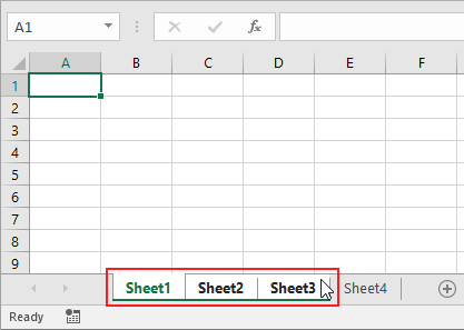
Now any format editing done on any of the selected three sheets will be copied to the other selected ones.
Here are all the observational notes using the formula in Excel.
Notes :
- This process is the most common practice.
- You can also copy format of any cell and apply to others using the Copy formatter option in Excel
Hope this article about How to format all worksheets in one go in Excel is explanatory. Find more articles on calculating values and related Excel formulas here. If you liked our blogs, share it with your friends on Facebook. And also you can follow us on Twitter and Facebook. We would love to hear from you, do let us know how we can improve, complement or innovate our work and make it better for you. Write to us at info@exceltip.com.
Related Articles :
50 Excel Shortcuts to Increase Your Productivity : Get faster at your tasks in Excel. These shortcuts will help you increase your work efficiency in Excel.
Replace text from end of a string starting from variable position : To replace text from the end of the string, we use the REPLACE function. The REPLACE function use the position of text in the string to replace.
How to Select Entire Column and Row Using Keyboard Shortcuts in Excel : Selecting cells is a very common function in Excel. Use Ctrl + Space to select columns and Shift + Space to select rows in Excel.
How to Insert Row Shortcut in Excel : Use Ctrl + Shift + = to open the Insert dialog box where you can insert row, column or cells in Excel.
How to Select Entire Column and Row Using Keyboard Shortcuts in Excel : Use Ctrl + Space to select whole column and Shift + Space to select whole row using keyboard shortcut in Excel
Excel Shortcut Keys for Merge and Center : This Merge and Center shortcut helps you quickly merge and unmerge cells.
Excel REPLACE vs SUBSTITUTE function: The REPLACE and SUBSTITUTE functions are the most misunderstood functions. To find and replace a given text we use the SUBSTITUTE function. Where REPLACE is used to replace a number of characters in string…
Popular Articles :
How to use the IF Function in Excel : The IF statement in Excel checks the condition and returns a specific value if the condition is TRUE or returns another specific value if FALSE.
How to use the VLOOKUP Function in Excel : This is one of the most used and popular functions of excel that is used to lookup value from different ranges and sheets.
How to use the SUMIF Function in Excel : This is another dashboard essential function. This helps you sum up values on specific conditions.
How to use the COUNTIF Function in Excel : Count values with conditions using this amazing function. You don’t need to filter your data to count specific values. Countif function is essential to prepare your dashboard.
This tutorial demonstrates how to apply conditional formatting to multiple sheets in Excel and Google Sheets.
In the latest versions of Excel, you can no longer select multiple sheets and then apply a conditional formatting rule to all the sheets at once. You need to do one sheet first, then copy the conditional formatting between sheets. Or, you can write a macro to repeat the conditional formatting on each sheet.
Apply Conditional Formatting to Multiple Sheets
Copy-Paste
- Select the sheet with the conditional formatting applied and right-click the cell with conditional formatting rule. Then click Copy (or use the keyboard shortcut CTRL + C).
- Next, click on the destination sheet and select the destination cell or cells. Right-click and choose Paste Special > Paste Format.
Format Painter
You can also copy the conditional formatting rule from one sheet to another with the Format Painter feature.
- Select the cell in the source sheet that has a conditional formatting rule and then, in the Ribbon, select Home > Clipboard > Format Painter.
- Click on the destination sheet and click on the cells or cell where you wish to apply the format.
Create a Macro to Apply Conditional Formatting Rule
While creating a new conditional formatting rule in Excel, you can record a macro to mimic the steps you take.
- In the Ribbon, select View > Macros > Record Macro.
OR, in the Ribbon, select Developer > Code > Record Macro.
Note: If you don’t see the Developer Ribbon, you’ll need to enable it.
- In the Record Macro dialog box, (1) type in a name for your macro and (2) make sure you select Personal Macro Workbook from the drop-down list. Then, (3) click OK to start recording.
- Once you have clicked OK, you can follow the steps to create the conditional formatting rule you require, and then click the stop button at the bottom of the screen to stop recording the macro.
- To run the macro on a different sheet, switch to that sheet and select the cell or cells you wish to apply the conditional formatting to.
- In the Ribbon, select View > Macros > View Macros.
OR Developer > Visual Basic > Macros
- Click on the Macro in the Macro name list and then select Run.
- You can run the macro on as many sheets as you require.
Note: You can view the code by selecting the macro in the Macro dialog box (shown above) and selecting Edit. This takes you to the Visual Basic Editor and enables you to view and/or edit your VBA code.
Apply Conditional Formatting to Multiple Sheets in Google Sheets
You can apply conditional formatting to multiple sheets in Google Sheets in the same way as you do in Excel.
Copy Conditional Formatting From One Cell
Copy-Paste
If you already have a cell or column with a Conditional Formatting rule set up, you can use Copy-Paste to copy the rule to another sheet.
- Right-click on a cell that has the conditional formatting rule applied to it and click Copy (or use the keyboard shortcut CTRL + C).
- Select the sheet you require and then select the cell or cells in that sheet where you wish to apply the conditional formatting rule. Select Paste special > Format only (or use the keyboard shortcut CTRL + ALT + V).
The conditional formatting rule will then be applied to the entire column you have selected.
Paint Format
If you already have a cell or column with a conditional formatting rule set up, you can use Paint Format to copy the rule to another column.
- Select the cell with the relevant conditional formatting rule. Then in the Menu, select Paint Format.
- Select the destination sheet, then highlight the cells to copy the conditional formatting rule to.
Often we come across workbooks that have similar formatting needs for multiple worksheets. For eg. you may have sales records spanning across 12 worksheets, one for each month. Now as a loyal reader of chandoo.org, you want to keep the formatting of all these worksheets consistent. So here is a quick tip to begin your work week.
- Just select all the different sheets (select one, then hold CTRL key and click on other sheet names).
- Now format any sheet and similar formatting will be applied to all selected sheets
- See this demo to understand:
The group & format technique is particularly useful when you,
- Want to apply same header / footer / print settings to multiple worksheets
- Want to write similar formulas in multiple worksheets (for eg. totals)
Do you use group sheets option?
I like to have consistent look & feel for all my worksheets. Especially if I am doing it for a client or for a product. So I find group sheets option pretty attractive and productive.
What about you? Do you use it? Share your tips & ideas with us.
More Quick Tips:
We have more than 60 quick excel tips that boost your productivity or introduce a new feature to simplify your work. Each of them is bite sized so you can learn quickly. Go on and consume a quick tip.
Share this tip with your colleagues

Get FREE Excel + Power BI Tips
Simple, fun and useful emails, once per week.
Learn & be awesome.
-
35 Comments -
Ask a question or say something… -
Tagged under
Excel 101, formatting, keyboard shortcuts, Learn Excel, quick tip, screencasts, spreadsheets, using excel
-
Category:
Learn Excel

Welcome to Chandoo.org
Thank you so much for visiting. My aim is to make you awesome in Excel & Power BI. I do this by sharing videos, tips, examples and downloads on this website. There are more than 1,000 pages with all things Excel, Power BI, Dashboards & VBA here. Go ahead and spend few minutes to be AWESOME.
Read my story • FREE Excel tips book


Excel School made me great at work.
5/5

From simple to complex, there is a formula for every occasion. Check out the list now.

Calendars, invoices, trackers and much more. All free, fun and fantastic.

Power Query, Data model, DAX, Filters, Slicers, Conditional formats and beautiful charts. It’s all here.

Still on fence about Power BI? In this getting started guide, learn what is Power BI, how to get it and how to create your first report from scratch.

- Excel for beginners
- Advanced Excel Skills
- Excel Dashboards
- Complete guide to Pivot Tables
- Top 10 Excel Formulas
- Excel Shortcuts
- #Awesome Budget vs. Actual Chart
- 40+ VBA Examples
Related Tips
35 Responses to “Formatting Multiple Worksheets? Use Group Sheets option to Speed up [Quick Tip]”
-
 Cyril Z. says:
 Wow!
I’ve never ever heared of that really powerful tip.
Thanks (as always) Cahndoo 🙂
-
I use it, for sure, but I’d also throw out the caution that, as soon as you’re done, UNGROUP them! I’ve destroyed more work by accidentally leaving sheets grouped than I care to remember.
It drives me crazy that every version of Excel has less contrast on the sheet tabs, which makes it harder and harder to tell if the sheets are grouped. I’m also not a big fan of how the grouped setting persists when the workbook is closed and re-opened.
It’s a great feature for making consistency, to be sure, but people need to be aware of the dangers of sheets being grouped when you forget to ungroup them. -
Josh says:
That is a very powerful tip, I spent hours just last week formatting things like this, except i was doing it one by one. Does anyone know if this works with formulas too?
-
Absolutely does, Josh. That’s why my caution. Entering formulas, deleting data, inserting & deleting rows… it all takes effect on the grouped sheets.
-
Josh says:
Oh, that could be disastrous… but also very very helpful.
If you look at the file name at the top of the workbook, it will tell say Book1 [Grouped] meaning that tabs are grouped. Just a quick tip to tell if tabs are grouped or not.
-
Ken- I think everyone had the problem you mentioned.. I know that drove me crazy every one in awhile when I would forget to ungroup them. Microsoft finally made it easier in Excel 2007, as soon as you click on another sheet, they ungroup — AS LONG AS ALL THE SHEETS HAD BEEN GROUPED ORIGINALLY. If you had some grouped and ungrouped then yes, you need to be very cautious. Another reason for using this is that grouping holds the column and row widths which you would have lost if you had just copied everything onto other sheets.
-
Aha! Thanks Patricia, I missed that improvement. I guess I always deal with a few subsheets at a time. (Usually have a control panel page in my applications that is formatted differently.) I still wish the contrast on the sheet tabs was more obvious though. 😉
-
Ken_M says:
Yes very powerful feature but not without signifigant downside if you need to have some sheets slightly different and you have not ungrouped them as you point out Ken. Patricia Another way to get consistent column widths is to do copy/paste special/column widths but this doesn’t help with rows — I believe there is another method to do this but I cannot recall it. Better contrast would help to alert you to the grouped selection
-
Amit kachroo says:
best trick dude::it’s really awesome
-
Brian says:
Chandoo mentions that this is useful if you «Want to apply same header / footer / print settings to multiple worksheets». I’ve used this before for entering data on multiple sheets but I have not been able to get it to work for headers/footers. I often receive files that need to be formatted for printing and this tip would be great if I could get it to work. Any suggestions?
-
Venus says:
I love this feature when 1) I remember to un-group the sheets, and 2) it actually works. I can’t even consider counting the number of times that I thought I’d reformatted all my worksheets only to move to another tab and find the formatting didn’t «stick». Personally I don’t like that sheets are un-grouped when I click on another sheet, I can’t think of the reason why, but many times I need to go to another sheet in the middle of all the formatting and they become ungrouped. I also become very frustrated when page or print settings don’t apply to all worksheets; it really seems to be a hit-or-miss thing. I must be doing something wrong somewhere 🙂
-
sanjeev says:
This function I would say, will only work perfectly if the data range is same in all the sheets which needs to be selected.
-
Narender kumar Nnada says:
I am totally new to excell and computer so found this sight highly useful
-
Bhupender Rao Y says:
It’s really useful tip for everyone……
-
Oatmeal says:
Great tool … have used it lots!
If you get one worksheet totally formatted, easiest way to clone them is to right click, Move or Copy Worksheet, click on what order you want it inserted click the little box at the bottom left that says «Create a Copy» and click OK — it’s cloned. Just do this a couple of times, then select the ones you already have cloned and do the right click, Move or Copy Worksheet and it clones that many at a time. -
Oatmeal says:
Brian, try this:
Select all the tabs you want to have the same footer, click on Page Layout ribbon, click the little box to the right of the Page Setup heading at the bottom of the Page Layout section and the old-fashioned Excel Page Setup option screen shows up.
Click on Headers & Footers, make the headers/footers that you want, and click OK. The headers/footers on all the selected tabs will be uniform!
Note: Make sure you unselect the tabs so any other changes you make don’t show up on all those tabs!
Cheers (from snowy Seattle!) -
Becky says:
Thank you for this lesson. I would like to learn how to apply VLOOKUP formula on a summary tab and the data are in each individual tab let’s just say 20 tabs within one Excel file. Is that possible?
Thanks.
-
archana says:
this was really a great tip .because i spent much by doing this on each sheet thanks chandoo.
-
Richard says:
First time on this site — will keep close eye on
-
Firestorm says:
I am a blind user of excel and this is an amazing tip, is there a way to do this with the keyboard? What about selecting non contineous worksheets in a workbook? Again using the keyboard, using the mouse makes it much simpler. Unfortunately not in a position to do so after losing eyesight.
-
@Firestorm
As a blind reader do you use «Reading» software to read Chandoo.org ?
Are the posts written in a style that is easily read?
Any other comments ?
Hui…
-
-
JoseLuis says:
Great tip Chandoo!
I have been teaching Excel since 2003 version and never heard of this one.
Thanks a lot. -
tink says:
This is an awesome tip I have been searching for daily for awhile now. Not sure why or how I found this site at this time but I am so thankful for it.
Thank you all for insights, tips and pointers. It has been most helpful. I will continue to frequent this site often as the position I recently acquired uses Excel extensively.
Again, thank you everyone, You are all awesome!
-
Chan says:
awesome tip..
is it possible to do conditional formatting for multiple sheets also?
-
Idris says:
Its Helpful,
But whenever i click on other sheet the grouping get back to compatibility mode, so is there any option to keep sheet grouping even if we click on other sheets. -
vilaskar says:
can you provide me Agewise based discounts tables in Excel
-
Carys says:
Hi- This is brilliant thank you! please can you help further? I have a workbook with 12 tabs (one for each month). I frequently need to make the same change to all, so I’m trying to use this method. Some cells are protected, so the group edit won’t work. Is there any way of unprotecting all 12 as a group, in order to make changes, and then re-protecting them please?
-
ken says:
I’m trying to handle something along these lines but with a twist. Backgorund, we areattempting to process logs of data in excell for debugging. e.g. 30 columns of data and hundreds or thousands of rows. Brute force approach, select column then apply ‘highlight cells rules’ to conditional format data in that column. Different columns get different rules to apply formatting. Ideally I could automate this with for instance a template to apply to a worksheet when I open the log file. I could define a macro but wonder if this is the recommended approach.
-
Abinash says:
Hi Chandoo,
I am finding short cut key to group or ungroup sheets. Can you help me? -
Bala says:
Wow! This helped.
You saved a lot of my time.
Thanks. -
saureign says:
in Excel 2010, it’s best to use ‘black’ theme. This way, the grouped sheets are clearly visible.
-
Rob says:
I’m trying to format multiple (110) sheets to fit on one page each, but when changing a scaling option on multiple sheets, the headers all change to the header on the first sheet selected. I want to scale each sheet (group of 110 sheets) to one page wide each without changing headers on any of the sheets. I can’t find an answer anywhere. Anyone happen to know a resolution?
-
Tsar Joseph Terungwa says:
A very useful and comprehended page, i love it