Excel sheet data from another sheet

Have you ever thought about what will you do if you need to transfer data from one Excel worksheet to another automatically?

or how will you update one Excel worksheet from another sheet, copy data from one sheet to another in Excel?

Keeping knowledge of these things is very important mainly when you are working with a large-size Excel worksheet having lots of data in it.

If you don’t have any clue about this, then this blog will help you out. As in this post, we will discuss how to copy data from one cell to another in Excel automatically?

Also, learn how to automatically update one Excel worksheet from another sheet, transfer data from one Excel worksheet to another automatically, and many more things in detail.

So, just go through this blog carefully.

Practical Scenario

Okay, first I should mention that I’m a complete amateur when it comes to excel. No VBA or macro experience, so if you’re not sure whether I know something yet, I probably don’t.

I have a workbook with 6 worksheets inside; one of the sheets is a master; it’s simply the other 6 sheets compiled into 1 big one. I need to set it up so that any new data entered into the new separate sheets is automatically entered into the master sheet, in the first blank row.

The columns are not the same across all the sheets. Hopefully, this will be easier for the pros here than it’s been for me, I’ve been banging my head against the wall on this one. I’ll be checking this thread religiously, so if you need any more information just let me know…

Thanks in advance for any help.

Source: https://ccm.net/forum/affich-1019001-automatically-update-master-worksheet-from-other-worksheets

Methods To Transfer Data From One Excel Workbook To Another

There are many different ways to transfer data from one Excel workbook to another and they are as follows:

Method #1: Automatically Update One Excel Worksheet From Another Sheet

In MS Excel workbook, we can easily update the data by linking one worksheet to another. This link is known as a dynamic formula that transfers data from one Excel workbook to another automatically.

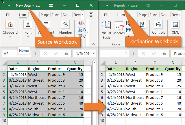
One Excel workbook is called the source worksheet, where this link carries the worksheet data automatically, and the other workbook is called the destination worksheet in which it automatically updates the worksheet data and contains the link formula.

The following are the two different points to link the Excel workbook data for the automatic updates.

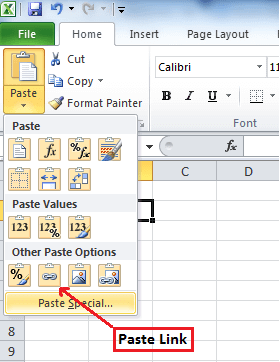
1) With the use of Copy and Paste option

In the source worksheet, select and copy the data that you want to link in another worksheet
Now in the destination worksheet, Paste the data where you have linked the cell source worksheet
After that choose the Paste Link menu from the Other Paste Options in the Excel workbook

Save all your work from the source worksheet before closing it

2) Manually enter the formula

Open your destination worksheet, tap to the cell that is having a link formula and put an equal sign (=) across it
Now go to the source sheet and tap to the cell which is having data. press Enter from your keyboard and save your tasks.

Note- Always remember one thing that the format of the source worksheet and the destination worksheet both are the same.

Method #2: Update Excel Spreadsheet With Data From Another Spreadsheet

To update Excel spreadsheets with data from another spreadsheet, just follow the points given below which will be applicable for the Excel version 2019, 2016, 2013, 2010, 2007.

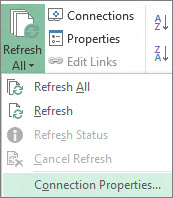
At first, go to the Data menu
Select Refresh All option

Here you have to see that when or how the connection is refreshed
Now click on any cell that contains the connected data
Again in the Data menu, click on the arrow which is next to Refresh All option and select Connection Properties

After that in the Usage menu, set the options that you want to change
On the Usage tab, set any options you want to change.

Note – If the size of the Excel data workbook is large, then I will recommend checking the Enable background refresh menu on a regular basis.

Method #3: How To Copy Data From One Cell To Another In Excel Automatically

To copy data from one cell to another in Excel, just go through the following points given below:

First, open the source worksheet and the destination worksheet.
In the source worksheet, navigate to the sheet that you want to move or copy
Now, click on the Home menu and choose the Format option
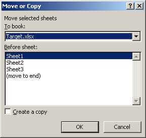
Then, select the Move Or Copy Sheet from the Organize Sheets part
After that, again in the Home menu choose the Format option in the cells group
Here in the Move Or Copy dialog option, select the target sheet and Excel will only display the open worksheets in the list

Else, if you want to copy the worksheet instead of moving, then kindly make a copy of the Excel workbook before

Lastly, select the OK button to copy or move the targeted Excel spreadsheet.

Method #4: How To Copy Data From One Sheet To Another In Excel Using Formula

You can copy data from one sheet to another in Excel using formula. Here are the steps to be followed:

For copy and paste the Excel cell in the present Excel worksheet, as for example; copy cell A1 to D5, you can just select the destination cell D5, then enter =A1 and press the Enter key to get the A1 value.
For copying and pasting cells from one worksheet to another worksheet such as copy cell A1 of Sheet1 to D5 of Sheet2, please select the cell D5 in Sheet2, then enter =Sheet1!A1 and press the Enter key to obtain the value.

Method #5: Copy Data From One Excel Sheet To Another Using Macros

With the help of macros, you can copy data from one worksheet to another but before this here are some important tips that you must take care of:

You should keep the file extension correctly in your Excel workbook.
It’s not necessary that your spreadsheet should be macro enable for doing the task.
The code that you choose can also be stored in a different worksheet.
As the codes already specify the details, so there is no need to activate the Excel workbook or cells first.
Thus, given below is the code for performing this task.

Sub OpenWorkbook()
‘Open a workbook
‘Open method requires full file path to be referenced.
Workbooks.Open “C:UsersusernameDocumentsNew Data.xlsx”

‘Open method has additional parameters
‘Workbooks.Open(FileName, UpdateLinks, ReadOnly, Format, Password, WriteResPassword, IgnoreReadOnlyRecommended, Origin, Delimiter, Editable, Notify, Converter, AddToMru, Local, CorruptLoad)

End Sub

Sub CloseWorkbook()
‘Close a workbook
Workbooks(“New Data.xlsx”).Close SaveChanges:=True
‘Close method has additional parameters
‘Workbooks.Close(SaveChanges, Filename, RouteWorkbook)

End Sub

Conclusion:

Well, I tried my level best to provide the best possible ways to transfer data from one Excel worksheet to another automatically. So from now on, you don’t have to worry about how to copy data from one cell to another in Excel automatically.

I hope you are satisfied with the above methods provided to you about Excel worksheet update.

Thus, make proper use of them and in the future also if you want to know about this, you can take the help of the specified solutions.

Priyanka is an entrepreneur & content marketing expert. She writes tech blogs and has expertise in MS Office, Excel, and other tech subjects. Her distinctive art of presenting tech information in the easy-to-understand language is very impressive. When not writing, she loves unplanned travels.

Источник

If your Excel spreadsheet has a lot of data, consider using different sheets to organize them. To pull data from another sheet in Excel, follow this guide.

Excel doesn’t just let you work in one spreadsheet—you can create multiple sheets within the same file. This is useful if you want to keep your data separated. If you were running a business, you could decide to have sales information for each month on separate sheets, for example.

What if you want to use some of the data from one sheet in another, however? You could copy and paste it across, but this can be time-consuming. If you make changes to any of the original data, the data you copied across won’t be updated.

The good news is that it’s not too tricky to use the data from one sheet in another. Here’s how to pull data from another sheet in Excel.

How to Pull Data From Another Sheet in Excel Using Cell References

You can pull data from one Excel sheet to another by using the relevant cell references. This is a simple way to get data from one sheet into another.

To pull data from another sheet by using cell references in Excel:

Click in the cell where you want the pulled data to appear.
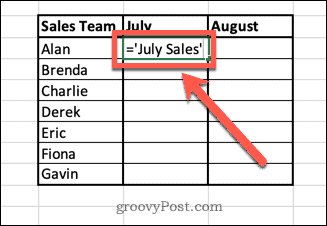
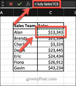
Type = (equals sign) followed by the name of the sheet you want to pull data from. If the name of the sheet is more than one word, enclose the sheet name in single quotes.
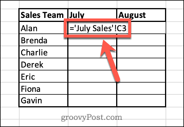
Type ! followed by the cell reference of the cell you want to pull.
Press Enter.
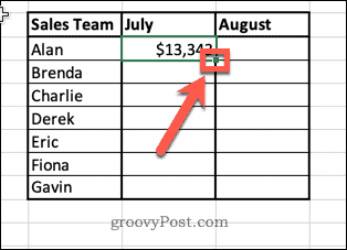
The value from your other sheet will now appear in the cell.
If you want to pull across more values, select the cell and hold the small square in the bottom-right corner of the cell.
Drag down to fill the remaining cells.

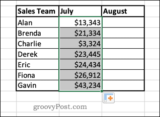
There is an alternative method that saves you from having to type in the cell references manually.

To pull data from another cell without typing the cell reference manually:

Click in the cell where you want the pulled data to appear.
Type = (equals sign) and then open the sheet from which you want to pull data.
Click on the cell containing the data that you want to pull across. You’ll see the formula change to include the reference to this cell.
Press Enter and the data will be pulled into your cell.

The method above works well if you’re not planning to do much with your data and just want to put it into a new sheet. However, there are some issues if you start to manipulate the data.

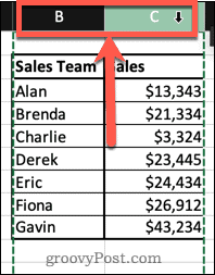
For example, if you sort the data in the July Sales sheet, the names of the sales team will also be rearranged.

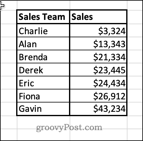
However, in the Sales Summary sheet, only the pulled data will change order. The other columns will remain the same, meaning that the sales are no longer aligned with the correct salesperson.

You can get around these issues by using the VLOOKUP function in Excel. Instead of pulling a value directly from a cell, this function pulls a value from a table that is in the same row as a unique identifier, such as the names in our example data. That means that even if the order of the original data changes, the data that is pulled will always remain the same.

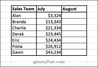
To use VLOOKUP to pull data from another sheet in Excel:

Click in the cell where you want the pulled data to appear.
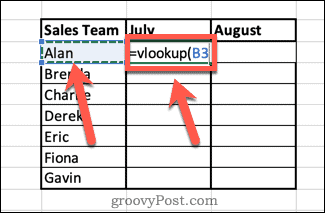
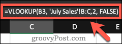
Type =VLOOKUP( then click on the cell to the left. This will be the reference that the VLOOKUP function will look for.
Type a comma, and then click on the sheet that you want to pull data from. Click and drag over the two columns that hold your data.
Type another comma, and then type the number of the column that contains the data you want to pull across. In this case, it’s the second column, so we would type 2.
Type another comma, then FALSE, then a final closed bracket to complete your formula. This ensures that the function looks for an exact match for your reference.
Press Enter. Your data will now appear in your cell.
If you want to pull across more values, select the cell and click and hold on the small square in the bottom right-hand corner of the cell.
Drag down to fill the remaining cells.
Now if you sort the original data, your pulled data will not change, since it is always looking for the data associated with each individual name.

Note that for this method to work, the unique identifiers (in this case, the names) must be in the first column of the range that you select.

Make Excel Work For You

There are hundreds of Excel functions that can take a lot of the grind out of your work and help you to do things quickly and easily. Knowing how to pull data from another sheet in Excel means you can say goodbye to endless copying and pasting.

Functions do have their limitations, however. As mentioned, this method will only work if your identifying data is in the first column. If your data is more complex, you’ll need to look into using other functions such as INDEX and MATCH.

VLOOKUP is a good place to start, however. If you’re having trouble with VLOOKUP, you should be able to troubleshoot VLOOKUP errors in Excel.

Источник

When working with excel sheets, you may have similar data that you are working with and which are in different excel sheets. Such data can be pulled from one of the sheets to another. This will save time in writing data in the columns or rows again.

To pull data from one excel sheet to another is the process of taking the data, be it in a column or a row, to another excel sheet. Once we pull values from another sheet, which is commonly done, we can save on time taken which we would otherwise keep in inserting the values in columns or rows.

Errors are minimized because while inserting the data all over again; you may omit some values, which will cause issues in the data set.

We have several procedures to follow to pull data from other sheets; the steps involved include the ones below;

Using Enter and Save

First, open a new excel sheet; in sheet 1, insert data as in the case below.

Leave the column with the estate as the header empty.

In sheet 2, enter the data as follows and save the excel sheet as «sheet2«

Using VLOOKUP Function

Having our sheets set with data values, we will now try and see if we can pull the values from sheet 2 to sheet 1. We have a function that we are going to use; the VLOOKUP function. This function will help us pull data values from sheet 2 to sheet 1. You can also pull data values from any other sheet you wish.

The formula that we will write on the formula bar of sheet 1 will be; = VLOOKUP (B3, ‘Sheet 2’! $B$3: $C$6, 2, 0). This formula on column B values will keep changing because B3 is only the first cell.

The formula will be able to pull the values of column C from sheet 2 upon clicking on the enter button, as in the case below.

The values will automatically be displayed in column C with the header Estate in both sheet 1 and sheet 1.

Using Advanced Filter in Excel

The Advanced Filter is among the easiest ways to use if you want to pull data from another sheet in Excel. For example, you can use it to pull data of customers and their payment details from one sheet and record it in the new worksheet. In this case, you can follow these simple steps:

1. Open the second spreadsheet and click on the Data button.

2. Select the Advanced option from the Sort and Filter commands.

3. A new dialogue box will show up. Select the Copy to another location option under the Action menu.

4. Next, fill in the List range box from the original worksheet. You can also click on the up-facing arrow to select the range directly.

5. Click on the Criteria range and select the data based on the criteria you want.

6. Finish by selecting the cell where you want the extracted data to appear and click the OK button.

If you wanted to pull data of customers who paid using their cards, you get your result showing only those who paid with cards in your preferred range of cells.

Using Combined INDEX And MATCH Functions

You can also combine INDEX and MATCH functions to pull data from one sheet to another based on your preferred criteria. The combination is among the powerful Excel hacks; hence, you can use it to extract customers’ payment details such as amount or payment mode. When using the combination, the MATCH function locates the matching value from the array of another sheet, while the INDEX function returns that value from the list. To pull data on customers’ amounts, you can follow these steps:

1. On a new sheet, select the cell you want to pull from the source sheet. For example, you can select cell D5, which has the customers’ value.

2. Write the following formula in the cell:

=INDEX(‘INDEX & MATCH Functions’!B5:E5,MATCH($B$5,’INDEX & MATCH Functions’!$B$4:$E$4,0))

3. Press the Enter key, and you will see the extracted amount in the new cell.

4. You can now use the cursor or Fill Handle to drag the formula down the column. This will automatically pull data from the source sheet to the new column.

Using the HLOOKUP Function

The HLOOKUP is a unique function to look up data horizontally and bring back the value. For instance, you can use it to pull out customers’ payment history into another worksheet through the following steps:

1. On the new sheet, select the cell with the dataset you want to pull out. For example, you can select cell E5.

2. Write the following formula in the cell and press the Enter button.

=HLOOKUP($B$5,’HLOOKUP Function’!$B$4:$E$8,Sheet4!D5+1,0)

3. You can now use the cursor or Fill Handle to drag the formula down the cells.

4. The function will pull out all the customers’ payment history from the source sheet and return the data to the new sheet.

Using Cell References

Of all the methods, using relevant cell references is the simplest way to pull data from one Excel sheet to another. Here, you can use these steps:

1. Select the cell where you want the extracted data to appear.

2. Type the equal sign (=) followed by the name of the sheet you want to pull data from. Enclose the sheet name in single quote marks if the name of the sheet is more than one word. Type the ‘!’ sign followed by the cell reference of the cell you to pull data from.

3. Press the Enter button, and the data from your source sheet will appear in the new cell.

4. You can now drag the Fill Handle (+) icon down the column to pull data from other remaining cells.

Источник

While working in Excel, we will often need to get values from another worksheet. This is possible by using the VLOOKUP function. In this tutorial, we will learn how to pull values from another worksheet in Excel, using VLOOKUP.

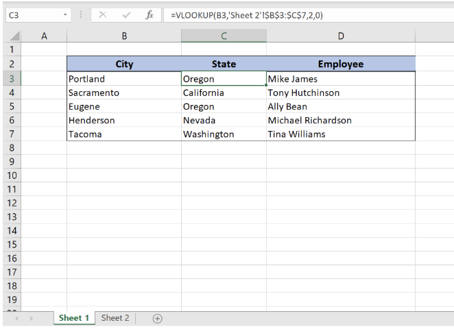
Figure 1. Final result

Syntax of the VLOOKUP formula

The generic formula for pulling values from another worksheet looks like:

=VLOOKUP(lookup_value, ’sheet_name’!range, col_index_num, range_lookup)

The parameters of the VLOOKUP function are:

lookup_value – a value that we want to find in another worksheet
’sheet_name’!range – a range in another worksheet in which we want to lookup
col_index_num – a column number in another worksheet from which we would like to pull a value
range_lookup – default value 0. This means that we want to find an exact match for a lookup value.

Setting up the Data

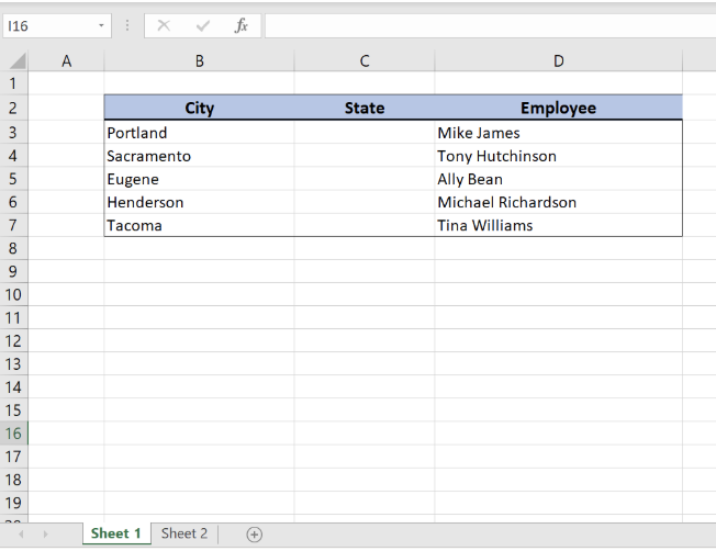Figure 2. “Sheet 1” in which we want to pull data

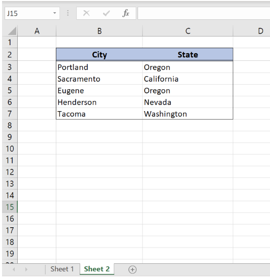Figure 3. Sheet 2 from which we want to pull data

We will now look at the example to explain in detail how this function works. Above all, let’s start with examining the structure of the data that we will use.

In “Sheet 1” we have a table in which we want to pull data, while in “Sheet2” we have the table from which we want to pull data. “Sheet 1” consists of “City” (column B), “State” (column C) and “Employee” (column D). “Sheet 2” consists of “City” (column B) and “State” (column C).

Get the State from Sheet 2 using VLOOKUP

Our goal is to obtain data from the “State” column in the second worksheet and populate it into the “State” column of the 1st worksheet. This will be done based on each corresponding city.

Figure 4. “Sheet 1” with pulled data in “State” column from “Sheet 2”

The formula looks like:

=VLOOKUP(B3,'Sheet 2'!$B$3:$C$7,2,0)

In our example, the lookup_value is the individual cell in “City” column. The parameter ’sheet_name’!range is ‘Sheet 2’!$B$3:$C$7 because we want to find value from the range B3:B7 in “Sheet 2”. Col_index_num has value 2, as we want to pull value from the second column of the range. Finally, range_lookup has value 0, because we want to find an exact match of “City” values.

Please note that we put absolute cell reference in table range ($ before B3:C7 range) as we must fix our lookup table.

To pull values from another worksheet, we need to follow these steps:

Select cell C3 and click on it
Insert the formula: =VLOOKUP(B3,'Sheet 2'!$B$3:$C$7,2,0)
Press enter
Drag the formula down to the other cells in the column by clicking and dragging the little “+” icon at the bottom-right of the cell.

As a result, we will get Oregon state in the cell B3. As you can see, the value of “City” in B3 on the “Sheet 1” is Portland, while in the “Sheet 2” state for Portland is Oregon. The function pulls this value and returns it to “Sheet 1” as a result.

Instant Connection to an Expert through our Excelchat Service:

Most of the time, the problem you will need to solve will be more complex than a simple application of a formula or function. If you want to save hours of research and frustration, try our live Excelchat service! Our Excel Experts are available 24/7 to answer any Excel question you may have. We guarantee a connection within 30 seconds and a customized solution within 20 minutes.

Are you still looking for help with the VLOOKUP function? View our comprehensive round-up of VLOOKUP function tutorials here.

Источник

Do you regularly work out of multiple Excel sheets? If so, you should know how to transfer data from one sheet to another automatically. This enormous time-saver doesn’t involve complicated formulas or add-ons, and it’s especially practical if you want to transfer specific data from one worksheet to another for reports. Below, you’ll learn two simple methods to copy data from one Excel sheet to another. These methods also link the sheets so that any changes you make to one sheet’s dataset automatically apply to the other. Finally, you’ll learn how to move data from one Excel sheet to another based on criteria by using the filter feature.

If you want to transfer data from one Google Sheet to another automatically, you can do that easily using Layer. Layer is a free add-on that allows you to share sheets or ranges of your main spreadsheet with different people. On top of that, you get to monitor and approve edits and changes made to the shared files before they’re merged back into your master file, giving you more control over your data.

Install the Layer Google Sheets Add-On today and Get Free Access to all the paid features, so you can start managing, automating, and scaling your processes on top of Google Sheets!

Two methods for automatically transferring data from one Excel worksheet to another

While there are various methods for transferring data from one Excel worksheet to another, the two simplest are the Copy and Paste Link and the Worksheet Reference methods.

How to Link Sheets in Excel?

Use Copy and Paste Link to automatically transfer data from one Excel worksheet to another

While you’re probably familiar with the standard Copy and Paste function, Excel offers multiple paste options. One of these is Link, which allows you to paste a value from another worksheet and link the pasted value to the copied value. In other words, if you change the original value you copied, the pasted value will automatically change as well.

These steps will show you how to use the Copy and Paste Link function:

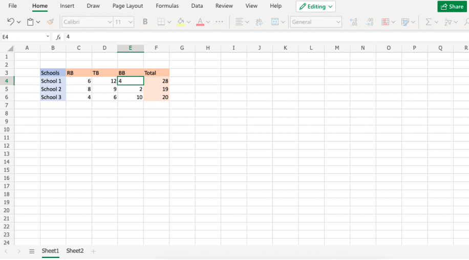
1. Open two spreadsheets containing the same simple dataset.

2. In sheet 1, select a cell and type Ctrl + C / Cmd + C to copy it.

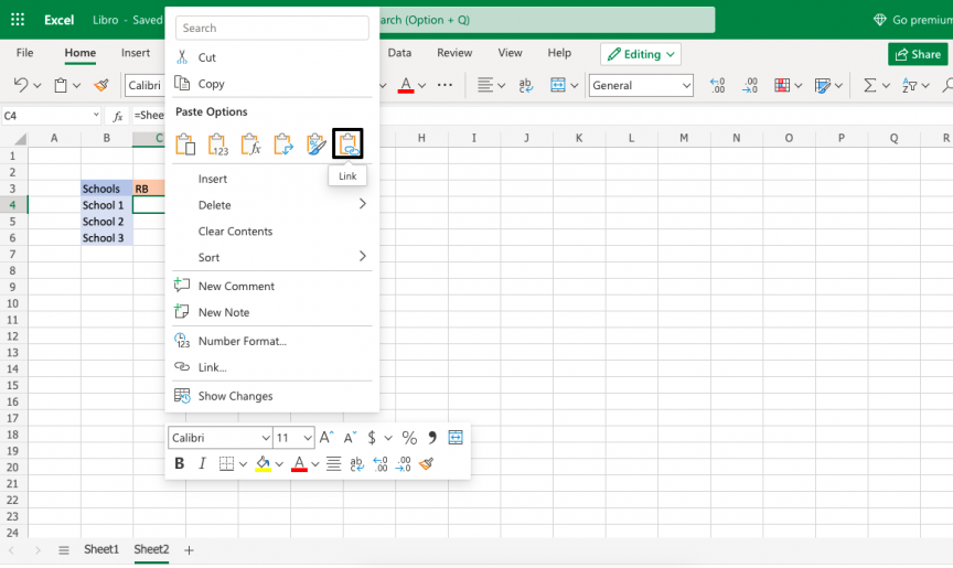
3. In sheet 2, right-click on the equivalent cell and go to the Paste > Link.

4. To prove they’re linked, return to sheet 1 and change the value in the cell you copied.

5. Finally, return to sheet 2 to see that the value has also changed.

How to VLOOKUP in Excel with Two Spreadsheets?

Sometimes our data may be spread out among different Excel sheets or workbooks. Here’s how to do VLOOKUP in Excel with two spreadsheets

Use worksheet reference to automatically transfer data from one Excel worksheet to another

This method is more manual than the Copy and Paste method but is equally simple and useful to know, just in case. The following steps will teach you how to use the worksheet reference method to transfer data from one Excel worksheet to another automatically:

1. Open two spreadsheets containing the same, simple dataset.

2. In sheet 2, double-click on a cell to the right of the dataset and type ‘=’.

3. Go to sheet 1, click any cell from the dataset, and press Enter.

You should automatically be returned to Sheet 2, where the cell previously containing ‘=’ now contains the value you chose to transfer from Sheet 1.

4. To prove they’re linked, return to Sheet 1 and change the value you chose to transfer.

Sheet 2 will automatically have changed the value to your chosen new value.

Move data from one Excel sheet to another based on criteria using the filter feature

In this example, you will learn how to filter data based on column criteria so that you keep only what you need. Then, you can copy and paste the data into a new sheet, as demonstrated in the above example.

1. Open a dataset on an Excel worksheet with filterable criteria.

2. Select the criteria column from which you want to filter and go to Data > Filter.

3. Click the small arrow beside the column header to open a drop-down menu.

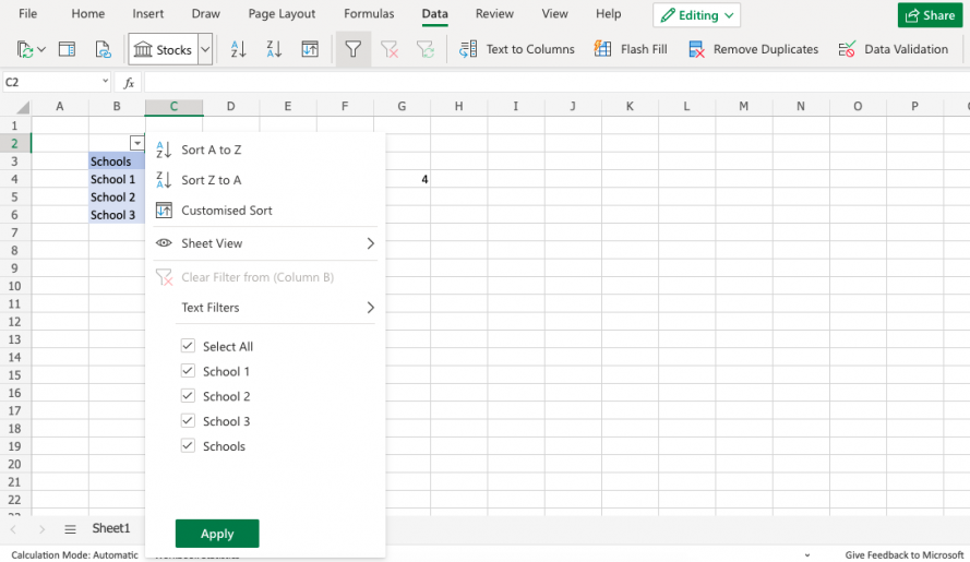
4. At the bottom of this menu, tick the box of the row(s) that you want to keep and click “Apply”.

You should now see only the data you wanted to keep.

To move this data to another sheet, follow the steps that show you how to copy and paste to automatically transfer data from one Excel worksheet to another.

Want to Boost Your Team’s Productivity and Efficiency?

Transform the way your team collaborates with Confluence, a remote-friendly workspace designed to bring knowledge and collaboration together. Say goodbye to scattered information and disjointed communication, and embrace a platform that empowers your team to accomplish more, together.

Key Features and Benefits:

Centralized Knowledge: Access your team’s collective wisdom with ease.
Collaborative Workspace: Foster engagement with flexible project tools.
Seamless Communication: Connect your entire organization effortlessly.
Preserve Ideas: Capture insights without losing them in chats or notifications.
Comprehensive Platform: Manage all content in one organized location.
Open Teamwork: Empower employees to contribute, share, and grow.
Superior Integrations: Sync with tools like Slack, Jira, Trello, and more.

Limited-Time Offer: Sign up for Confluence today and claim your forever-free plan, revolutionizing your team’s collaboration experience.

Conclusion

So, if you didn’t know before how useful it is to link and transfer data from one Excel worksheet to another automatically, you do now. With the Copy and Paste Link and worksheet reference method, you can transfer data effectively in a matter of minutes. What’s more, you’ll never have to worry about these spreadsheets again — any update in one will be automatically transferred to the other immediately. You can also move data from one Excel sheet to another based on criteria by filtering your data to transfer only what you want. This is great for transferring data for important reports, saving you lots of time from unnecessary copy and pasting, and report editing.

If you work with multiple worksheets in Excel and found this article helpful, you should also check out these related posts: How to do VLOOKUP in excel with two spreadsheets, and How to use IMPORTRANGE in Google Sheets.

Hady is Content Lead at Layer.

Hady has a passion for tech, marketing, and spreadsheets. Besides his Computer Science degree, he has vast experience in developing, launching, and scaling content marketing processes at SaaS startups.

Originally published Feb 3 2022, Updated Mar 22 2023

Источник

Practical Scenario

Methods To Transfer Data From One Excel Workbook To Another

Method #1: Automatically Update One Excel Worksheet From Another Sheet

Method #2: Update Excel Spreadsheet With Data From Another Spreadsheet

Method #3: How To Copy Data From One Cell To Another In Excel Automatically

Method #4: How To Copy Data From One Sheet To Another In Excel Using Formula

Method #5: Copy Data From One Excel Sheet To Another Using Macros

Recommended Solution: MS Excel Repair & Recovery Tool

Steps to Utilize MS Excel Repair & Recovery Tool:

Conclusion:

How to Pull Data From Another Sheet in Excel Using Cell References

Make Excel Work For You

Using Enter and Save

Using VLOOKUP Function

Using Advanced Filter in Excel

Using Combined INDEX And MATCH Functions

Using the HLOOKUP Function

Using Cell References

Syntax of the VLOOKUP formula

Setting up the Data

Get the State from Sheet 2 using VLOOKUP

Instant Connection to an Expert through our Excelchat Service:

Two methods for automatically transferring data from one Excel worksheet to another

How to Link Sheets in Excel?

Use Copy and Paste Link to automatically transfer data from one Excel worksheet to another

How to VLOOKUP in Excel with Two Spreadsheets?

Use worksheet reference to automatically transfer data from one Excel worksheet to another

Move data from one Excel sheet to another based on criteria using the filter feature

Want to Boost Your Team’s Productivity and Efficiency?

Conclusion

А вот еще интересные статьи: