Try:
.Formula = "='" & strProjectName & "'!" & Cells(2, 7).Address
If your worksheet name (strProjectName) has spaces, you need to include the single quotes in the formula string.
If this does not resolve it, please provide more information about the specific error or failure.
Update
In comments you indicate you’re replacing spaces with underscores. Perhaps you are doing something like:
strProjectName = Replace(strProjectName," ", "_")
But if you’re not also pushing that change to the Worksheet.Name property, you can expect these to happen:
- The file browse dialog appears
- The formula returns
#REFerror
The reason for both is that you are passing a reference to a worksheet that doesn’t exist, which is why you get the #REF error. The file dialog is an attempt to let you correct that reference, by pointing to a file wherein that sheet name does exist. When you cancel out, the #REF error is expected.
So you need to do:
Worksheets(strProjectName).Name = Replace(strProjectName," ", "_")
strProjectName = Replace(strProjectName," ", "_")
Then, your formula should work.
Excel for Microsoft 365 Excel for Microsoft 365 for Mac Excel for the web Excel 2021 Excel 2021 for Mac Excel 2019 Excel 2019 for Mac Excel 2016 Excel 2016 for Mac Excel 2013 Excel for iPad Excel for iPhone Excel for Android tablets Excel 2010 Excel 2007 Excel for Mac 2011 Excel for Android phones Excel Starter 2010 More…Less
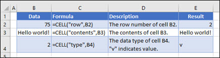
The CELL function returns information about the formatting, location, or contents of a cell. For example, if you want to verify that a cell contains a numeric value instead of text before you perform a calculation on it, you can use the following formula:
=IF(CELL(«type»,A1)=»v»,A1*2,0)
This formula calculates A1*2 only if cell A1 contains a numeric value, and returns 0 if A1 contains text or is blank.
Note: Formulas that use CELL have language-specific argument values and will return errors if calculated using a different language version of Excel. For example, if you create a formula containing CELL while using the Czech version of Excel, that formula will return an error if the workbook is opened using the French version. If it is important for others to open your workbook using different language versions of Excel, consider either using alternative functions or allowing others to save local copies in which they revise the CELL arguments to match their language.
Syntax
CELL(info_type, [reference])
The CELL function syntax has the following arguments:
|
Argument |
Description |
|---|---|
|
info_type Required |
A text value that specifies what type of cell information you want to return. The following list shows the possible values of the Info_type argument and the corresponding results. |
|
reference Optional |
The cell that you want information about. If omitted, the information specified in the info_type argument is returned for cell selected at the time of calculation. If the reference argument is a range of cells, the CELL function returns the information for active cell in the selected range. Important: Although technically reference is optional, including it in your formula is encouraged, unless you understand the effect its absence has on your formula result and want that effect in place. Omitting the reference argument does not reliably produce information about a specific cell, for the following reasons:
|
info_type values
The following list describes the text values that can be used for the info_type argument. These values must be entered in the CELL function with quotes (» «).
|
info_type |
Returns |
|---|---|
|
«address» |
Reference of the first cell in reference, as text. |
|
«col» |
Column number of the cell in reference. |
|
«color» |
The value 1 if the cell is formatted in color for negative values; otherwise returns 0 (zero). Note: This value is not supported in Excel for the web, Excel Mobile, and Excel Starter. |
|
«contents» |
Value of the upper-left cell in reference; not a formula. |
|
«filename» |
Filename (including full path) of the file that contains reference, as text. Returns empty text («») if the worksheet that contains reference has not yet been saved. Note: This value is not supported in Excel for the web, Excel Mobile, and Excel Starter. |
|
«format» |
Text value corresponding to the number format of the cell. The text values for the various formats are shown in the following table. Returns «-» at the end of the text value if the cell is formatted in color for negative values. Returns «()» at the end of the text value if the cell is formatted with parentheses for positive or all values. Note: This value is not supported in Excel for the web, Excel Mobile, and Excel Starter. |
|
«parentheses» |
The value 1 if the cell is formatted with parentheses for positive or all values; otherwise returns 0. Note: This value is not supported in Excel for the web, Excel Mobile, and Excel Starter. |
|
«prefix» |
Text value corresponding to the «label prefix» of the cell. Returns single quotation mark (‘) if the cell contains left-aligned text, double quotation mark («) if the cell contains right-aligned text, caret (^) if the cell contains centered text, backslash () if the cell contains fill-aligned text, and empty text («») if the cell contains anything else. Note: This value is not supported in Excel for the web, Excel Mobile, and Excel Starter. |
|
«protect» |
The value 0 if the cell is not locked; otherwise returns 1 if the cell is locked. Note: This value is not supported in Excel for the web, Excel Mobile, and Excel Starter. |
|
«row» |
Row number of the cell in reference. |
|
«type» |
Text value corresponding to the type of data in the cell. Returns «b» for blank if the cell is empty, «l» for label if the cell contains a text constant, and «v» for value if the cell contains anything else. |
|
«width» |
Returns an array with 2 items. The 1st item in the array is the column width of the cell, rounded off to an integer. Each unit of column width is equal to the width of one character in the default font size. The 2nd item in the array is a Boolean value, the value is TRUE if the column width is the default or FALSE if the width has been explicitly set by the user. Note: This value is not supported in Excel for the web, Excel Mobile, and Excel Starter. |
CELL format codes
The following list describes the text values that the CELL function returns when the Info_type argument is «format» and the reference argument is a cell that is formatted with a built-in number format.
|
If the Excel format is |
The CELL function returns |
|---|---|
|
General |
«G» |
|
0 |
«F0» |
|
#,##0 |
«,0» |
|
0.00 |
«F2» |
|
#,##0.00 |
«,2» |
|
$#,##0_);($#,##0) |
«C0» |
|
$#,##0_);[Red]($#,##0) |
«C0-« |
|
$#,##0.00_);($#,##0.00) |
«C2» |
|
$#,##0.00_);[Red]($#,##0.00) |
«C2-« |
|
0% |
«P0» |
|
0.00% |
«P2» |
|
0.00E+00 |
«S2» |
|
# ?/? or # ??/?? |
«G» |
|
m/d/yy or m/d/yy h:mm or mm/dd/yy |
«D4» |
|
d-mmm-yy or dd-mmm-yy |
«D1» |
|
d-mmm or dd-mmm |
«D2» |
|
mmm-yy |
«D3» |
|
mm/dd |
«D5» |
|
h:mm AM/PM |
«D7» |
|
h:mm:ss AM/PM |
«D6» |
|
h:mm |
«D9» |
|
h:mm:ss |
«D8» |
Note: If the info_type argument in the CELL function is «format» and you later apply a different format to the referenced cell, you must recalculate the worksheet (press F9) to update the results of the CELL function.
Examples
Need more help?
You can always ask an expert in the Excel Tech Community or get support in the Answers community.
See Also
Change the format of a cell
Create or change a cell reference
ADDRESS function
Add, change, find or clear conditional formatting in a cell
Need more help?
Вставка формулы со ссылками в стиле A1 и R1C1 в ячейку (диапазон) из кода VBA Excel. Свойства Range.FormulaLocal и Range.FormulaR1C1Local.
Свойство Range.FormulaLocal
FormulaLocal — это свойство объекта Range, которое возвращает или задает формулу на языке пользователя, используя ссылки в стиле A1.
В качестве примера будем использовать диапазон A1:E10, заполненный числами, которые необходимо сложить построчно и результат отобразить в столбце F:

Примеры вставки формул суммирования в ячейку F1:
|
Range(«F1»).FormulaLocal = «=СУММ(A1:E1)» Range(«F1»).FormulaLocal = «=СУММ(A1;B1;C1;D1;E1)» |
Пример вставки формул суммирования со ссылками в стиле A1 в диапазон F1:F10:
|
Sub Primer1() Dim i As Byte For i = 1 To 10 Range(«F» & i).FormulaLocal = «=СУММ(A» & i & «:E» & i & «)» Next End Sub |
В этой статье я не рассматриваю свойство Range.Formula, но если вы решите его применить для вставки формулы в ячейку, используйте англоязычные функции, а в качестве разделителей аргументов — запятые (,) вместо точек с запятой (;):
|
Range(«F1»).Formula = «=SUM(A1,B1,C1,D1,E1)» |
После вставки формула автоматически преобразуется в локальную (на языке пользователя).
Свойство Range.FormulaR1C1Local
FormulaR1C1Local — это свойство объекта Range, которое возвращает или задает формулу на языке пользователя, используя ссылки в стиле R1C1.
Формулы со ссылками в стиле R1C1 можно вставлять в ячейки рабочей книги Excel, в которой по умолчанию установлены ссылки в стиле A1. Вставленные ссылки в стиле R1C1 будут автоматически преобразованы в ссылки в стиле A1.
Примеры вставки формул суммирования со ссылками в стиле R1C1 в ячейку F1 (для той же таблицы):
|
‘Абсолютные ссылки в стиле R1C1: Range(«F1»).FormulaR1C1Local = «=СУММ(R1C1:R1C5)» Range(«F1»).FormulaR1C1Local = «=СУММ(R1C1;R1C2;R1C3;R1C4;R1C5)» ‘Ссылки в стиле R1C1, абсолютные по столбцам и относительные по строкам: Range(«F1»).FormulaR1C1Local = «=СУММ(RC1:RC5)» Range(«F1»).FormulaR1C1Local = «=СУММ(RC1;RC2;RC3;RC4;RC5)» ‘Относительные ссылки в стиле R1C1: Range(«F1»).FormulaR1C1Local = «=СУММ(RC[-5]:RC[-1])» Range(«F2»).FormulaR1C1Local = «=СУММ(RC[-5];RC[-4];RC[-3];RC[-2];RC[-1])» |
Пример вставки формул суммирования со ссылками в стиле R1C1 в диапазон F1:F10:
|
‘Ссылки в стиле R1C1, абсолютные по столбцам и относительные по строкам: Range(«F1:F10»).FormulaR1C1Local = «=СУММ(RC1:RC5)» ‘Относительные ссылки в стиле R1C1: Range(«F1:F10»).FormulaR1C1Local = «=СУММ(RC[-5]:RC[-1])» |
Так как формулы с относительными ссылками и относительными по строкам ссылками в стиле R1C1 для всех ячеек столбца F одинаковы, их можно вставить сразу, без использования цикла, во весь диапазон.
|
vigor Пользователь Сообщений: 172 |
Добрый вечер.Коротко суть проблемы. |
|
Kuzmich Пользователь Сообщений: 7998 |
ActiveCell.Formula = «=SUM(ActiveSheet(«111»).Range(Cells(1,переменная), _ |
|
vigor Пользователь Сообщений: 172 |
Не работает.Сами попробуйте, я так уже експериментировал |
|
nerv  Пользователь Сообщений: 3071 |
ActiveCell.Formula = «=СУММ(» & Range(«A2»).Address & «,» & Range(«A3»).Address & «)» |
|
Hugo Пользователь Сообщений: 23249 |
Идиотская конструкция получилась… With Sheets(«111») |
|
Hugo Пользователь Сообщений: 23249 |
Лист потерялся, не заметил… ActiveCell.Formula = «=SUM(111!» & Cells(1, m).Address & «,111!» & Cells(5, n).Address & «)» |
|
Hugo Пользователь Сообщений: 23249 |
|
|
Насчет ActiveSheet(«111») согласен Prist.Спешил.Все остальное работает спасибо ребята |
|
|
vigor Пользователь Сообщений: 172 |
Ребятки посоветуйте книгу по RibbonX,или прикольную статейку в Нете.Буду благодарен |
|
nerv Пользователь Сообщений: 3071 |
Но его радость была бы не полной. Позвольте добавить идиотизма : ) ActiveCell.Formula = «=СУММ(‘» & Sheets(«111»).Name & «‘!» & Range(«A2»).Address & «,» & Range(«A3»).Address & «)» |
|
nerv Пользователь Сообщений: 3071 |
#11 02.07.2011 10:50:13 {quote}{login=The_Prist}{date=02.07.2011 09:58}{thema=Re: }{post}{quote}{login=nerv}{date=01.07.2011 11:22}{thema=}{post}Но его радость была бы не полной. Позвольте добавить идиотизма : ) ActiveCell.Formula = «=СУММ(‘» & Sheets(«111»).Name & «‘!» & Range(«A2»).Address & «,» & Range(«A3»).Address & «)»{/post}{/quote}А Вы уверены, что в таком случае суммироваться будут ячейки с одного только листа «111»? Специально заменил СУММ на SUM, т.к. в таком случае локализация не влияет и формула не выдаст ИМЯ.{/post}{/quote}не уверен Чебурашка стал символом олимпийских игр. А чего достиг ты? |


Return to Excel Formulas List
Download Example Workbook
Download the example workbook
This tutorial will demonstrate how to use a cell value in a formula in Excel and Google Sheets.
Cell Value as a Cell Reference
The INDIRECT Function is useful when you want to convert a text string in a cell into a valid cell reference, be it the cell address or a range name.
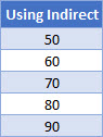
=INDIRECT(D4)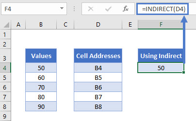
The INDIRECT Function will look at the text string in cell D4 which in this case is B4 – it will then use the text string as a valid cell reference and return the value that is contained in B4 – in this instance, 50.
If you copy the formula down, the D4 will change to D5, D6 etc, and the correct value from column B will be returned.
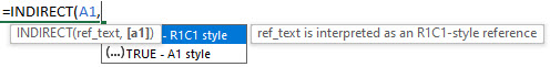
The Syntax of the INDIRECT Function is:
=INDIRECT(reference, reference style)The reference style can be either R1C1 style or can be the more familiar A1 style. If you omit this argument, the A1 style is assumed.
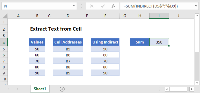
SUM Function With the INDIRECT Function
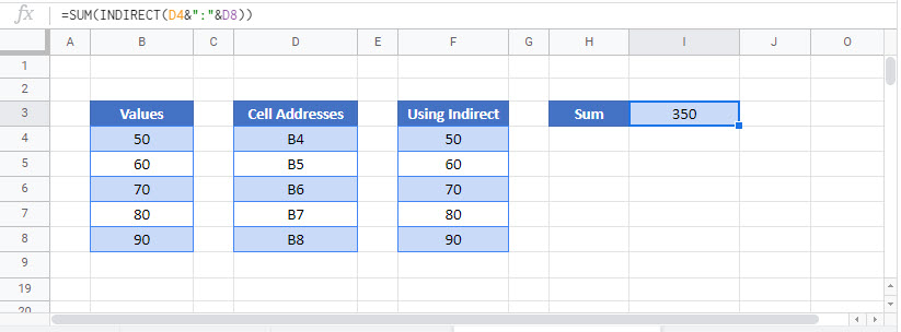
We can also use the INDIRECT function with the SUM Function to add up the values in column B by using the text strings in column D.
Click in H4 and type the following formula.
=SUM(INDIRECT(D4&":"&D8))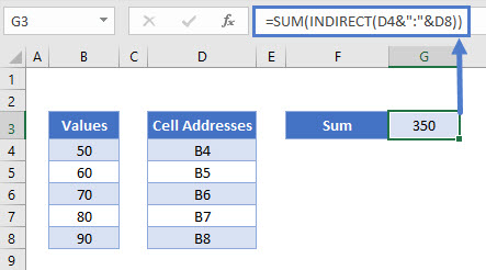
INDIRECT Function With Range Names in Excel
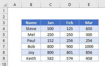
Now let’s look at an example of using the INDIRECT Function with Named Ranges.
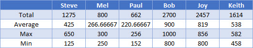
Consider the following worksheet where the sales figures are shown for a period of 3 months for several Sales Reps.
- Select the Range B3:E9.
- In the Ribbon, select Formulas > Create from Selection.
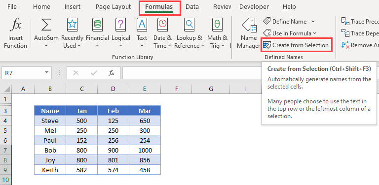
- Make sure that the Top row and the Left Column check boxes are ticked and click OK.
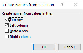
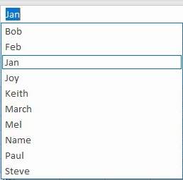
- Excel will now have created range names based on your selection.
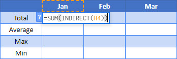
- Click in H4 and set up a table as shown below.
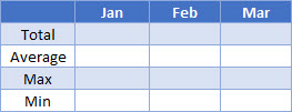
- In I4, type the following formula:
=SUM(INDIRECT(I3)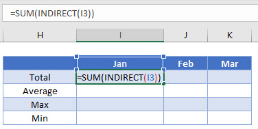
- Press Enter to complete the formula.
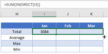
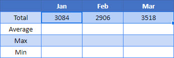
- Drag the formula across to column K.
- The formula will change from picking up I3 to picking up J3 (the Feb range name) and then K3 (the March range name).
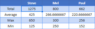
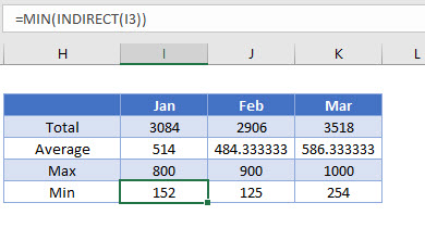
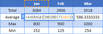
- Repeat the process for the AVERAGE, MAX and MIN functions.
- We can then amend the names in row 3 to get the totals for 3 of the sales reps. The formulas will automatically pick up the correct values due to the INDIRECT
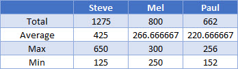
- Type in the name of the remaining reps in the adjacent column and drag the formulas across to get their sales figures.
Cell Value as a Cell Reference in Google Sheets
Using the INDIRECT Function in Google sheets works the same way as it does in Excel.
INDIRECT Function with Range Names in Google Sheets
Named Ranges work similar to Excel in Google Sheets.
- In the Menu, select Data>Named Ranges.
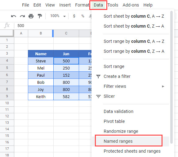
- Type in the name or the range, and then select the range.
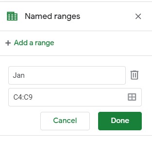
- Click Done.
- Repeat the process for all the months, and all the sales reps
- Once you have created the range names, you can use them in the same way as you used them in Excel.
- Drag the formula across to February and March.
- Repeat for the AVERAGE, MIN and MAX functions.
- We can then amend the names in row 3 to get the totals for 3 of the sales reps. The formulas will automatically pick up the correct values due to the INDIRECT