
I found a similar solution to this question in c# How to Select all the cells in a worksheet in Excel.Range object of c#?
What is the process to do this in VBA?
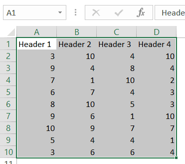
I select data normally by using «ctrl+shift over arrow, down arrow» to select an entire range of cells. When I run this in a macro it codes out A1:Q398247930, for example. I need it to just be
.SetRange Range("A1:whenever I run out of rows and columns")
I could easily do it myself without a macro, but I’m trying to make the entire process a macro, and this is just a piece of it.
Sub sort()
    'sort Macro
    Range("B2").Select
    ActiveWorkbook.Worksheets("Master").sort.SortFields.Clear
    ActiveWorkbook.Worksheets("Master").sort.SortFields.Add Key:=Range("B2"), _
      SortOn:=xlSortOnValues, Order:=xlAscending, DataOption:=xlSortNormal
    With ActiveWorkbook.Worksheets("Master").sort
        .SetRange Range("A1:whenever I run out of rows and columns")
        .Header = xlNo
        .MatchCase = False
        .Orientation = xlTopToBottom
        .SortMethod = xlPinYin
        .Apply
    End With
End Sub
edit:
There are other parts where I might want to use the same code but the range is say «C3:End of rows & columns». Is there a way in VBA to get the location of the last cell in the document?
asked Jul 30, 2013 at 18:50
![]()
C. TewaltC. Tewalt
2,2612 gold badges29 silver badges47 bronze badges
I believe you want to find the current region of A1 and surrounding cells — not necessarily all cells on the sheet.
If so — simply use…
Range(«A1»).CurrentRegion
answered Jul 30, 2013 at 19:17
![]()
ExcelExpertExcelExpert
3522 silver badges4 bronze badges
1
You can simply use cells.select to select all cells in the worksheet. You can get a valid address by saying Range(Cells.Address).
If you want to find the last Used Range where you have made some formatting change or entered a value into you can call ActiveSheet.UsedRange and select it from there. Hope that helps.
![]()
June7
19.5k8 gold badges24 silver badges33 bronze badges
answered Jul 30, 2013 at 19:11
![]()
chanceachancea
5,8083 gold badges28 silver badges39 bronze badges
2
you can use all cells as a object like this :
Dim x as Range
Set x = Worksheets("Sheet name").Cells
X is now a range object that contains the entire worksheet
answered Apr 15, 2015 at 11:47
![]()
you have a few options here:
- Using the UsedRange property
- find the last row and column used
- use a mimic of shift down and shift right
I personally use the Used Range and find last row and column method most of the time.
Here’s how you would do it using the UsedRange property:
Sheets("Sheet_Name").UsedRange.Select
This statement will select all used ranges in the worksheet, note that sometimes this doesn’t work very well when you delete columns and rows.
The alternative is to find the very last cell used in the worksheet
Dim rngTemp As Range
Set rngTemp = Cells.Find("*", SearchOrder:=xlByRows, SearchDirection:=xlPrevious)
If Not rngTemp Is Nothing Then
    Range(Cells(1, 1), rngTemp).Select
End If
What this code is doing:
- Find the last cell containing any value
- select cell(1,1) all the way to the last cell
![]()
answered Jul 30, 2013 at 20:32
![]()
Derek ChengDerek Cheng
5353 silver badges8 bronze badges
3
Another way to select all cells within a range, as long as the data is contiguous, is to use Range("A1", Range("A1").End(xlDown).End(xlToRight)).Select.
answered Mar 29, 2019 at 19:38
![]()
I would recommend recording a macro, like found in this post;
Excel VBA macro to filter records
But if you are looking to find the end of your data and not the end of the workbook necessary, if there are not empty cells between the beginning and end of your data, I often use something like this;
R = 1
Do While Not IsEmpty(Sheets("Sheet1").Cells(R, 1))
    R = R + 1
Loop
Range("A5:A" & R).Select 'This will give you a specific selection
You are left with R = to the number of the row after your data ends. This could be used for the column as well, and then you could use something like Cells(C , R).Select, if you made C the column representation.
![]()
answered Jul 30, 2013 at 19:25
![]()
MakeCentsMakeCents
7321 gold badge5 silver badges15 bronze badges
2
Sub SelectAllCellsInSheet(SheetName As String)
    lastCol = Sheets(SheetName).Range("a1").End(xlToRight).Column
    Lastrow = Sheets(SheetName).Cells(1, 1).End(xlDown).Row
    Sheets(SheetName).Range("A1", Sheets(SheetName).Cells(Lastrow, lastCol)).Select
End Sub
To use with ActiveSheet:
Call SelectAllCellsInSheet(ActiveSheet.Name)
answered Mar 14, 2017 at 20:57
![]()
Yehia AmerYehia Amer
5985 silver badges11 bronze badges
Here is what I used, I know it could use some perfecting, but I think it will help others…
''STYLING''

Dim sheet As Range

' Find Number of rows used
Dim Final As Variant
    Final = Range("A1").End(xlDown).Row

' Find Last Column
Dim lCol As Long
    lCol = Cells(1, Columns.Count).End(xlToLeft).Column

Set sheet = ActiveWorkbook.ActiveSheet.Range("A" & Final & "", Cells(1, lCol ))
With sheet
    .Interior.ColorIndex = 1
End With
answered Mar 16, 2019 at 4:29
![]()
I have found that the Worksheet «.UsedRange» method is superior in many instances to solve this problem.
I struggled with a truncation issue that is a normal behaviour of the «.CurrentRegion» method. Using [ Worksheets(«Sheet1»).Range(«A1»).CurrentRegion ] does not yield the results I desired when the worksheet consists of one column with blanks in the rows (and the blanks are wanted). In this case, the «.CurrentRegion» will truncate at the first record. I implemented a work around but recently found an even better one; see code below that allows copying the whole set to another sheet or to identify the actual address (or just rows and columns):
Sub mytest_GetAllUsedCells_in_Worksheet()
    Dim myRange

    Set myRange = Worksheets("Sheet1").UsedRange
    'Alternative code:  set myRange = activesheet.UsedRange

   'use msgbox or debug.print to show the address range and counts
   MsgBox myRange.Address
   MsgBox myRange.Columns.Count
   MsgBox myRange.Rows.Count

  'Copy the Range of data to another sheet
  'Note: contains all the cells with that are non-empty
   myRange.Copy (Worksheets("Sheet2").Range("A1"))
   'Note:  transfers all cells starting at "A1" location.
   '       You can transfer to another area of the 2nd sheet
   '       by using an alternate starting location like "C5".

End Sub
answered May 2, 2019 at 19:38
![]()
Maybe this might work:
Sh.Range(«A1», Sh.Range(«A» & Rows.Count).End(xlUp))
answered Oct 31, 2014 at 18:38
![]()
Refering to the very first question, I am looking into the same.
The result I get, recording a macro, is, starting by selecting cell A76:
Sub find_last_row()
    Range("A76").Select
    Range(Selection, Selection.End(xlDown)).Select
End Sub
answered Aug 7, 2015 at 12:40
![]()
Хитрости »
26 Июль 2015 77731 просмотров
Все начинающие изучать VBA сталкиваются с тем, что записанные через макрорекордер коды пестрят методами Select и Activate.
Если не знакомы с работой макрорекордера — Что такое макрос и где его искать?
Это значительно ухудшает читабельность кода и, как ни странно — быстродействие. Но есть недостатки и куда более критичные. Если код выполняется достаточно долго и он постоянно что-то выделяет — пользователь может заскучать и забыться и начнет тыкать мышкой по листам и ячейкам, выделяя не то, что выделил ранее код. Что повлечет ошибки логики. Т.е. код может и выполнится, но совершенно не так, как ожидалось. Поэтому избавляться от Select и Activate необходимо везде, где это возможно.
Для начала рассмотрим два кода, выполняющие одни те же действия — запись в ячейку А3 листа Лист2 слова «Привет». При этом сам код запускается с Лист1 и после выполнения код Лист1 должен остаться активным. Чтобы сделать эти действия вручную потребуется сначала перейти на Лист2, выделить ячейку А3, записать в неё слово «Привет» и вернуться на Лист1. Поэтому запись макрорекордером этих действий приведет к такому коду:
Sub Макрос1()
    Sheets("Лист2").Select            'выделяем Лист2
    Range("A3").Select                'выделяем ячейку А3
    ActiveCell.FormulaR1C1 = "Привет" 'записываем слово Привет
    Range("A4").Select                'после нажатия Enter автоматически выделяется ячейка А4
    Sheets("Лист1").Select            'возвращаемся на Лист1
End Sub
Нигде не говорится, что в большинстве случаев все эти Select и Activate в кодах не нужны. Однако вышеприведенный код можно значительно улучшить, если убрать все ненужные Select и Activate:
Sub Макрос1()
    Sheets("Лист2").Range("A3").FormulaR1C1 = "Привет"
End Sub
Как видно, вместо 5-ти строк кода получилась одна строка. Которая выполняет ту же задачу, что и код из 5-ти строк.
Прежде чем понять как правильно избавляться от лишнего давайте разберемся зачем же тогда VBA записывает эти Select и Activate? Как ни странно, но здесь все очень просто. VBA просто не знает, что Вы будете делать после того, как выделили Лист2. И когда Вы переходите на Лист2 — VBA записывает именно переход(его активацию, выделение). Когда выделяете ячейку — так же именно это действие записывает VBA. Захотите ли Вы затем выделить еще что-то, или закрасить ячейку, или записать в неё формулу/значение — VBA не знает. Поэтому в дальнейшем VBA работает именно с выделенным объектом Selection на активном листе.
Но при написании кода вручную или при правке записанного рекордером мы уже вольны в выборе и знаем, чего хотели добиться и какие действия нам точно не нужны.
Итак, чтобы записать в ячейку слово «Привет» рекордер предложит нам такой код:
Sub Макрос1()
    Range("A3").Select                'выделяем ячейку А3
    ActiveCell.FormulaR1C1 = "Привет" 'записываем слово Привет
    Range("A4").Select                'после нажатия Enter автоматически выделяется ячейка А4
End Sub
однако выделять ячейку(Range(«A3»).Select) совершенно необязательно. Значит один Select уже лишний. После этого идет обращение к активной ячейке — ActiveCell. .FormulaR1C1 = «Привет» означает запись значения «Привет» в эту ячейку.
Пусть не смущает FormulaR1C1 — VBA всегда так указывает запись и значения и формулы. Т.к. перед словом «Привет» нет знака равно — то это значение.
Т.к. ActiveCell является обращением к выделенной ячейке, а выделили мы до этого А3, значит их можно просто «сократить»:
Sub Макрос1()
    Range("A3").FormulaR1C1 = "Привет"
    Range("A4").Select                'после нажатия Enter автоматически выделяется ячейка А4
End Sub
Теперь у нас код получился короче и понятнее. Однако остался один Select: Range(«A4»).Select. Если нет необходимости выделять ячейку А4 после записи в А3 значения, то надо просто удалить эту строку и после выполнения кода активной будет та ячейка, которая была выделена до выполнения(т.е. выделенная ячейка просто не изменится). Таким образом мы с трех строк сократим код до 1-ой:
Sub Макрос1()
    Range("A3").FormulaR1C1 = "Привет"
End Sub
Теперь несложно догадаться, что с листами все в точности так же. Sheets(«Лист2»).Select — Select хоть и не нужен, но и ActiveSheet после него нет. Здесь необходимо знать некоторую иерархию в Excel. Сначала идет сам Excel — Application, потом книга — Workbook. В книгу входят рабочие листы(Worksheets), а уже в листах — ячейки и диапазоны — Range и Cells(Application ->Workbook ->Worksheet ->Range). Если перед Range или Cells не указывать явно лист: Range(«A3»).FormulaR1C1 = «Привет», то значение будет записано на активный лист. Подробнее можно прочесть в статье: Как обратиться к диапазону из VBA
Маленький нюанс: если сокращаем обращение к объектам, то Select-ов быть не должно вообще. Иначе есть шанс получить ошибку «Subscript out of range»:
буквально это означает, что указанный индекс вне досягаемости. А появляется эта ошибка потому, что нельзя выделить ячейку НЕактивного листа или лист НЕактивной книги. Легко эту ошибку получить например в таком коде:Sub Макрос2() Windows("Книга3").Activate 'здесь появится ошибка, т.к. пытаемся выделить лист в Книга2 'а на данный момент активной является Книга3 Windows("Книга2").Sheets("Лист3").Select End SubОшибка обязательно появится, т.к. сначала мы активировали кодом книгу «Книга3», а потом пытаемся активировать лист НЕактивной на этот момент книги «Книга2». А это сделать невозможно без активации той книги, в которой активируемый лист. Т.е. активация должна происходить именно последовательно: Книга ->Лист ->Ячейка. И никак иначе, если мы хотим активировать именно конкретную ячейку конкретного листа в конкретной книге.
И пример с ячейками:Sub Макрос2() Sheets("Лист3").Select 'здесь появится ошибка, т.к. пытаемся выделить ячейку на листе "Лист1" 'а на данный момент активным является Лист3 Sheets("Лист1").Range("C7").Select End SubТак же такая ошибка может появиться и по той простой причине, что указанного листа или книги нет(листа с указанным именем нет в данной книге или книга, к которой обращаемся просто закрыта).

Еще небольшой пример оптимизации:
Sub Макрос2()
    Windows("Книга3").Activate
    Sheets("Лист3").Select
    Range("C7").Select
    ActiveCell.FormulaR1C1 = "Привет"
    Range("C7").Select
    Selection.Font.Bold = True
    With Selection.Interior
        .Pattern = xlSolid
        .PatternColorIndex = xlAutomatic
        .Color = 65535
        .TintAndShade = 0
        .PatternTintAndShade = 0
    End With
End Sub
Этот код записывает в ячейку С7 Лист3 книги «Книга3» слово «Привет», потом делает жирным шрифт и назначает желтый цвет заливке. Убираем активацию книги, листа и ячейки, заменив их прямым обращением:
Workbooks("Книга3").Sheets("Лист3").Range("C7").FormulaR1C1 = "Привет"
далее делаем для ячейки жирный шрифт:
Workbooks("Книга3").Sheets("Лист3").Range("C7").Font.Bold = True
и цвет заливки:
With Workbooks("Книга3").Sheets("Лист3").Range("C7").Interior
    .Pattern = xlSolid
    .PatternColorIndex = xlAutomatic
    .Color = 65535
    .TintAndShade = 0
    .PatternTintAndShade = 0
End With
Тут есть нюанс. Windows необходимо всегда заменять на Workbooks — в кодах я сделал именно так. Если этого не сделать, то получите ошибку 438 — объект не поддерживает данное свойство или метод(object dos’t support this property or metod), т.к. коллекция Windows не содержит определения для Sheets.
Важный момент: лучше всегда указать имя книги вместе с расширением(.xlsx, xlsm, .xls и т.д.). Если в настройках ОС Windows(Панель управления —Параметры папок -вкладка Вид —Скрывать расширения для зарегистрированных типов файлов) указано скрывать расширения — то указывать расширение не обязательно — Workbooks(«Книга2»). Но и ошибки не будет, если его указать. Однако, если пункт «Скрывать расширения для зарегистрированных типов файлов» отключен, то указание Workbooks(«Книга2») обязательно приведет к ошибке.
Вместо Workbooks(«Книга3.xlsx») можно использовать обращение к активной книге или книге, в которой расположен код. Обращение к Лист3 активной книги, когда активен Лист2 или другой:
ActiveWorkbook.Sheets("Лист3").Range("A1").Value = "Привет"
Но бывают случаи, когда необходимо производить действия исключительно в той книге, в которой сам код. И не зависеть при этом от того, какая книга активна в данный момент и как она называется. Ведь в процессе книга может быть переименована. За это отвечает ThisWorkbook:
ThisWorkbook.Sheets("Лист3").Range("A1").Value = "Привет"
ActiveWorkbook — действия с активной на момент выполнения кода книгой
ThisWorkbook — действия с книгой, в которой записан код
Однако так же бывают случаи, когда необходимо обращаться к новой книге или листу, которые были созданы в процессе работы кода. В таком случае необходимо использовать переменные:
Sub NewBook()
    'объявляем переменную для дальнейшего обращения
    Dim wbNewBook As Workbook
    'создаем книгу
    Set wbNewBook = Workbooks.Add
    'теперь можно обращаться к wbNewBook как к любой другой книге
    'но уже не указывая её имя
    wbNewBook.Sheets(1).Range("A1").Value = "Привет"
    'Sheets(1) - обращение к листу по его порядковому номеру
    '(отсчет с начинается с 1 слева)
End Sub
Sub NewSheet()
    'объявляем переменную для дальнейшего обращения
    Dim wsNewSheet As Worksheet
    'добавляем новый лист в активную книгу
    Set wsNewSheet = ActiveWorkbook.Sheets.Add
    'теперь можно обращаться к wsNewSheet как к любому другому листу
    'но уже не указывая его имя или индекс
    wsNewSheet.Range("A1").Value = "Привет"
End Sub
Не везде Activate лишний
Но есть и такие свойства и методы, которые требуют обязательной активации книги/листа. Одним из таких свойств является свойство окна FreezePanes(Закрепление областей):
Sub Freeze_Panes()
    ThisWorkbook.Activate
    Sheets(2).Activate
    Range("B2").Select
    ActiveWindow.FreezePanes = True
End Sub
В этом коде нельзя убирать Select и Activate, т.к. свойство FreezePanes применяется исключительно к активному листу и активной ячейке, потому что является оно именно методом окна, а не листа или ячейки.
Так же сюда можно отнести свойства: Split, SplitColumn, SplitHorizontal и им подобные. Иными словами все свойства, которые работают исключительно с активным окном приложения, а не с объектами напрямую.
Так же см.:
Что такое макрос и где его искать?
Что такое модуль? Какие бывают модули?
Как обратиться к диапазону из VBA
Что такое переменная и как правильно её объявить?
Статья помогла? Поделись ссылкой с друзьями!
![]() Видеоуроки
Видеоуроки
Поиск по меткам
Access
apple watch
Multex
Power Query и Power BI
VBA управление кодами
Бесплатные надстройки
Дата и время
Записки
ИП
Надстройки
Печать
Политика Конфиденциальности
Почта
Программы
Работа с приложениями
Разработка приложений
Росстат
Тренинги и вебинары
Финансовые
Форматирование
Функции Excel
акции MulTEx
ссылки
статистика
When working with Excel, most of your time is spent in the worksheet area – dealing with cells and ranges.
And if you want to automate your work in Excel using VBA, you need to know how to work with cells and ranges using VBA.
There are a lot of different things you can do with ranges in VBA (such as select, copy, move, edit, etc.).
So to cover this topic, I will break this tutorial into sections and show you how to work with cells and ranges in Excel VBA using examples.
Let’s get started.
All the codes I mention in this tutorial need to be placed in the VB Editor. Go to the ‘Where to Put the VBA Code‘ section to know how it works.
If you’re interested in learning VBA the easy way, check out my Online Excel VBA Training.
Selecting a Cell / Range in Excel using VBA
To work with cells and ranges in Excel using VBA, you don’t need to select it.
In most of the cases, you are better off not selecting cells or ranges (as we will see).
Despite that, it’s important you go through this section and understand how it works. This will be crucial in your VBA learning and a lot of concepts covered here will be used throughout this tutorial.
So let’s start with a very simple example.
Selecting a Single Cell Using VBA
If you want to select a single cell in the active sheet (say A1), then you can use the below code:
Sub SelectCell()
Range("A1").Select
End Sub
The above code has the mandatory ‘Sub’ and ‘End Sub’ part, and a line of code that selects cell A1.
Range(“A1”) tells VBA the address of the cell that we want to refer to.
Select is a method of the Range object and selects the cells/range specified in the Range object. The cell references need to be enclosed in double quotes.
This code would show an error in case a chart sheet is an active sheet. A chart sheet contains charts and is not widely used. Since it doesn’t have cells/ranges in it, the above code can’t select it and would end up showing an error.
Note that since you want to select the cell in the active sheet, you just need to specify the cell address.
But if you want to select the cell in another sheet (let’s say Sheet2), you need to first activate Sheet2 and then select the cell in it.
Sub SelectCell()
Worksheets("Sheet2").Activate
Range("A1").Select
End Sub
Similarly, you can also activate a workbook, then activate a specific worksheet in it, and then select a cell.
Sub SelectCell()
Workbooks("Book2.xlsx").Worksheets("Sheet2").Activate
Range("A1").Select
End Sub
Note that when you refer to workbooks, you need to use the full name along with the file extension (.xlsx in the above code). In case the workbook has never been saved, you don’t need to use the file extension.
Now, these examples are not very useful, but you will see later in this tutorial how we can use the same concepts to copy and paste cells in Excel (using VBA).
Just as we select a cell, we can also select a range.
In case of a range, it could be a fixed size range or a variable size range.
In a fixed size range, you would know how big the range is and you can use the exact size in your VBA code. But with a variable-sized range, you have no idea how big the range is and you need to use a little bit of VBA magic.
Let’s see how to do this.
Selecting a Fix Sized Range
Here is the code that will select the range A1:D20.
Sub SelectRange()
Range("A1:D20").Select
End Sub
Another way of doing this is using the below code:
Sub SelectRange()
Range("A1", "D20").Select
End Sub
The above code takes the top-left cell address (A1) and the bottom-right cell address (D20) and selects the entire range. This technique becomes useful when you’re working with variably sized ranges (as we will see when the End property is covered later in this tutorial).
If you want the selection to happen in a different workbook or a different worksheet, then you need to tell VBA the exact names of these objects.
For example, the below code would select the range A1:D20 in Sheet2 worksheet in the Book2 workbook.
Sub SelectRange()
Workbooks("Book2.xlsx").Worksheets("Sheet1").Activate
Range("A1:D20").Select
End Sub
Now, what if you don’t know how many rows are there. What if you want to select all the cells that have a value in it.
In these cases, you need to use the methods shown in the next section (on selecting variably sized range).
Selecting a Variably Sized Range
There are different ways you can select a range of cells. The method you choose would depend on how the data is structured.
In this section, I will cover some useful techniques that are really useful when you work with ranges in VBA.
Select Using CurrentRange Property
In cases where you don’t know how many rows/columns have the data, you can use the CurrentRange property of the Range object.
The CurrentRange property covers all the contiguous filled cells in a data range.
Below is the code that will select the current region that holds cell A1.
Sub SelectCurrentRegion()
Range("A1").CurrentRegion.Select
End Sub
The above method is good when you have all data as a table without any blank rows/columns in it.
But in case you have blank rows/columns in your data, it will not select the ones after the blank rows/columns. In the image below, the CurrentRegion code selects data till row 10 as row 11 is blank.
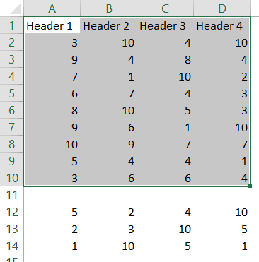
In such cases, you may want to use the UsedRange property of the Worksheet Object.
Select Using UsedRange Property
UsedRange allows you to refer to any cells that have been changed.
So the below code would select all the used cells in the active sheet.
Sub SelectUsedRegion()
ActiveSheet.UsedRange.Select
End Sub
Note that in case you have a far-off cell that has been used, it would be considered by the above code and all the cells till that used cell would be selected.
Select Using the End Property
Now, this part is really useful.
The End property allows you to select the last filled cell. This allows you to mimic the effect of Control Down/Up arrow key or Control Right/Left keys.
Let’s try and understand this using an example.
Suppose you have a dataset as shown below and you want to quickly select the last filled cells in column A.
The problem here is that data can change and you don’t know how many cells are filled. If you have to do this using keyboard, you can select cell A1, and then use Control + Down arrow key, and it will select the last filled cell in the column.
Now let’s see how to do this using VBA. This technique comes in handy when you want to quickly jump to the last filled cell in a variably-sized column
Sub GoToLastFilledCell()
Range("A1").End(xlDown).Select
End Sub
The above code would jump to the last filled cell in column A.
Similarly, you can use the End(xlToRight) to jump to the last filled cell in a row.
Sub GoToLastFilledCell()
Range("A1").End(xlToRight).Select
End Sub
Now, what if you want to select the entire column instead of jumping to the last filled cell.
You can do that using the code below:
Sub SelectFilledCells()
Range("A1", Range("A1").End(xlDown)).Select
End Sub
In the above code, we have used the first and the last reference of the cell that we need to select. No matter how many filled cells are there, the above code will select all.
Remember the example above where we selected the range A1:D20 by using the following line of code:
Range(“A1″,”D20”)
Here A1 was the top-left cell and D20 was the bottom-right cell in the range. We can use the same logic in selecting variably sized ranges. But since we don’t know the exact address of the bottom-right cell, we used the End property to get it.
In Range(“A1”, Range(“A1”).End(xlDown)), “A1” refers to the first cell and Range(“A1”).End(xlDown) refers to the last cell. Since we have provided both the references, the Select method selects all the cells between these two references.
Similarly, you can also select an entire data set that has multiple rows and columns.
The below code would select all the filled rows/columns starting from cell A1.
Sub SelectFilledCells()
Range("A1", Range("A1").End(xlDown).End(xlToRight)).Select
End Sub
In the above code, we have used Range(“A1”).End(xlDown).End(xlToRight) to get the reference of the bottom-right filled cell of the dataset.
Difference between Using CurrentRegion and End
If you’re wondering why use the End property to select the filled range when we have the CurrentRegion property, let me tell you the difference.
With End property, you can specify the start cell. For example, if you have your data in A1:D20, but the first row are headers, you can use the End property to select the data without the headers (using the code below).
Sub SelectFilledCells()
Range("A2", Range("A2").End(xlDown).End(xlToRight)).Select
End Sub
But the CurrentRegion would automatically select the entire dataset, including the headers.
So far in this tutorial, we have seen how to refer to a range of cells using different ways.
Now let’s see some ways where we can actually use these techniques to get some work done.
Copy Cells / Ranges Using VBA
As I mentioned at the beginning of this tutorial, selecting a cell is not necessary to perform actions on it. You will see in this section how to copy cells and ranges without even selecting these.
Let’s start with a simple example.
Copying Single Cell
If you want to copy cell A1 and paste it into cell D1, the below code would do it.
Sub CopyCell()
Range("A1").Copy Range("D1")
End Sub
Note that the copy method of the range object copies the cell (just like Control +C) and pastes it in the specified destination.
In the above example code, the destination is specified in the same line where you use the Copy method. If you want to make your code even more readable, you can use the below code:
Sub CopyCell()
Range("A1").Copy Destination:=Range("D1")
End Sub
The above codes will copy and paste the value as well as formatting/formulas in it.
As you might have already noticed, the above code copies the cell without selecting it. No matter where you’re on the worksheet, the code will copy cell A1 and paste it on D1.
Also, note that the above code would overwrite any existing code in cell D2. If you want Excel to let you know if there is already something in cell D1 without overwriting it, you can use the code below.
Sub CopyCell()
If Range("D1") <> "" Then
Response = MsgBox("Do you want to overwrite the existing data", vbYesNo)
End If
If Response = vbYes Then
Range("A1").Copy Range("D1")
End If
End Sub
Copying a Fix Sized Range
If you want to copy A1:D20 in J1:M20, you can use the below code:
Sub CopyRange()
Range("A1:D20").Copy Range("J1")
End Sub
In the destination cell, you just need to specify the address of the top-left cell. The code would automatically copy the exact copied range into the destination.
You can use the same construct to copy data from one sheet to the other.
The below code would copy A1:D20 from the active sheet to Sheet2.
Sub CopyRange()
Range("A1:D20").Copy Worksheets("Sheet2").Range("A1")
End Sub
The above copies the data from the active sheet. So make sure the sheet that has the data is the active sheet before running the code. To be safe, you can also specify the worksheet’s name while copying the data.
Sub CopyRange()
Worksheets("Sheet1").Range("A1:D20").Copy Worksheets("Sheet2").Range("A1")
End Sub
The good thing about the above code is that no matter which sheet is active, it will always copy the data from Sheet1 and paste it in Sheet2.
You can also copy a named range by using its name instead of the reference.
For example, if you have a named range called ‘SalesData’, you can use the below code to copy this data to Sheet2.
Sub CopyRange()
Range("SalesData").Copy Worksheets("Sheet2").Range("A1")
End Sub
If the scope of the named range is the entire workbook, you don’t need to be on the sheet that has the named range to run this code. Since the named range is scoped for the workbook, you can access it from any sheet using this code.
If you have a table with the name Table1, you can use the below code to copy it to Sheet2.
Sub CopyTable()
Range("Table1[#All]").Copy Worksheets("Sheet2").Range("A1")
End Sub
You can also copy a range to another Workbook.
In the following example, I copy the Excel table (Table1), into the Book2 workbook.
Sub CopyCurrentRegion()
Range("Table1[#All]").Copy Workbooks("Book2.xlsx").Worksheets("Sheet1").Range("A1")
End Sub
This code would work only if the Workbook is already open.
Copying a Variable Sized Range
One way to copy variable sized ranges is to convert these into named ranges or Excel Table and the use the codes as shown in the previous section.
But if you can’t do that, you can use the CurrentRegion or the End property of the range object.
The below code would copy the current region in the active sheet and paste it in Sheet2.
Sub CopyCurrentRegion()
Range("A1").CurrentRegion.Copy Worksheets("Sheet2").Range("A1")
End Sub
If you want to copy the first column of your data set till the last filled cell and paste it in Sheet2, you can use the below code:
Sub CopyCurrentRegion()
Range("A1", Range("A1").End(xlDown)).Copy Worksheets("Sheet2").Range("A1")
End Sub
If you want to copy the rows as well as columns, you can use the below code:
Sub CopyCurrentRegion()
Range("A1", Range("A1").End(xlDown).End(xlToRight)).Copy Worksheets("Sheet2").Range("A1")
End Sub
Note that all these codes don’t select the cells while getting executed. In general, you will find only a handful of cases where you actually need to select a cell/range before working on it.
Assigning Ranges to Object Variables
So far, we have been using the full address of the cells (such as Workbooks(“Book2.xlsx”).Worksheets(“Sheet1”).Range(“A1”)).
To make your code more manageable, you can assign these ranges to object variables and then use those variables.
For example, in the below code, I have assigned the source and destination range to object variables and then used these variables to copy data from one range to the other.
Sub CopyRange()
Dim SourceRange As Range
Dim DestinationRange As Range
Set SourceRange = Worksheets("Sheet1").Range("A1:D20")
Set DestinationRange = Worksheets("Sheet2").Range("A1")
SourceRange.Copy DestinationRange
End Sub
We start by declaring the variables as Range objects. Then we assign the range to these variables using the Set statement. Once the range has been assigned to the variable, you can simply use the variable.
Enter Data in the Next Empty Cell (Using Input Box)
You can use the Input boxes to allow the user to enter the data.
For example, suppose you have the data set below and you want to enter the sales record, you can use the input box in VBA. Using a code, we can make sure that it fills the data in the next blank row.
Sub EnterData()
Dim RefRange As Range
Set RefRange = Range("A1").End(xlDown).Offset(1, 0)
Set ProductCategory = RefRange.Offset(0, 1)
Set Quantity = RefRange.Offset(0, 2)
Set Amount = RefRange.Offset(0, 3)
RefRange.Value = RefRange.Offset(-1, 0).Value + 1
ProductCategory.Value = InputBox("Product Category")
Quantity.Value = InputBox("Quantity")
Amount.Value = InputBox("Amount")
End Sub
The above code uses the VBA Input box to get the inputs from the user, and then enters the inputs into the specified cells.
Note that we didn’t use exact cell references. Instead, we have used the End and Offset property to find the last empty cell and fill the data in it.
This code is far from usable. For example, if you enter a text string when the input box asks for quantity or amount, you will notice that Excel allows it. You can use an If condition to check whether the value is numeric or not and then allow it accordingly.
Looping Through Cells / Ranges
So far we can have seen how to select, copy, and enter the data in cells and ranges.
In this section, we will see how to loop through a set of cells/rows/columns in a range. This could be useful when you want to analyze each cell and perform some action based on it.
For example, if you want to highlight every third row in the selection, then you need to loop through and check for the row number. Similarly, if you want to highlight all the negative cells by changing the font color to red, you need to loop through and analyze each cell’s value.
Here is the code that will loop through the rows in the selected cells and highlight alternate rows.
Sub HighlightAlternateRows()
Dim Myrange As Range
Dim Myrow As Range
Set Myrange = Selection
For Each Myrow In Myrange.Rows
If Myrow.Row Mod 2 = 0 Then
Myrow.Interior.Color = vbCyan
End If
Next Myrow
End Sub
The above code uses the MOD function to check the row number in the selection. If the row number is even, it gets highlighted in cyan color.
Here is another example where the code goes through each cell and highlights the cells that have a negative value in it.
Sub HighlightAlternateRows()
Dim Myrange As Range
Dim Mycell As Range
Set Myrange = Selection
For Each Mycell In Myrange
If Mycell < 0 Then
Mycell.Interior.Color = vbRed
End If
Next Mycell
End Sub
Note that you can do the same thing using Conditional Formatting (which is dynamic and a better way to do this). This example is only for the purpose of showing you how looping works with cells and ranges in VBA.
Where to Put the VBA Code
Wondering where the VBA code goes in your Excel workbook?
Excel has a VBA backend called the VBA editor. You need to copy and paste the code in the VB Editor module code window.
Here are the steps to do this:
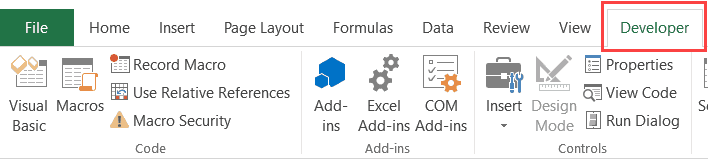
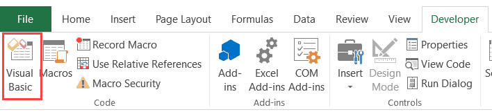
- Go to the Developer tab.

- Click on the Visual Basic option. This will open the VB editor in the backend.
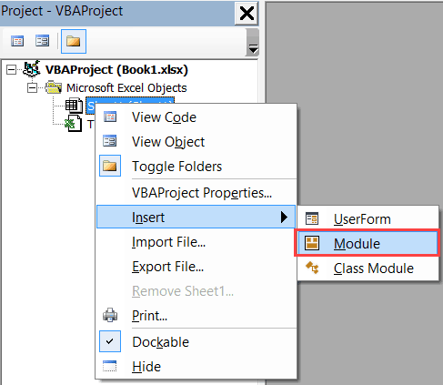
- In the Project Explorer pane in the VB Editor, right-click on any object for the workbook in which you want to insert the code. If you don’t see the Project Explorer, go to the View tab and click on Project Explorer.
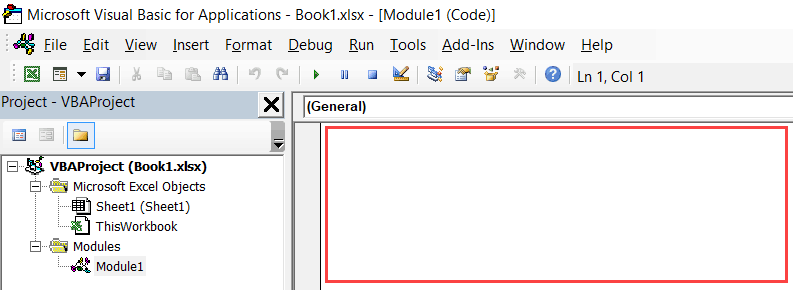
- Go to Insert and click on Module. This will insert a module object for your workbook.

- Copy and paste the code in the module window.

You May Also Like the Following Excel Tutorials:
- Working with Worksheets using VBA.
- Working with Workbooks using VBA.
- Creating User-Defined Functions in Excel.
- For Next Loop in Excel VBA – A Beginner’s Guide with Examples.
- How to Use Excel VBA InStr Function (with practical EXAMPLES).
- Excel VBA Msgbox.
- How to Record a Macro in Excel.
- How to Run a Macro in Excel.
- How to Create an Add-in in Excel.
- Excel Personal Macro Workbook | Save & Use Macros in All Workbooks.
- Excel VBA Events – An Easy (and Complete) Guide.
- Excel VBA Error Handling.
- How to Sort Data in Excel using VBA (A Step-by-Step Guide).
- 24 Useful Excel Macro Examples for VBA Beginners (Ready-to-use).
![]()
Download Article
![]()
Download Article
This wikiHow teaches you how to start using Visual Basic procedures to select data in Microsoft Excel. As long as you’re familiar with basic VB scripting and using more advanced features of Excel, you’ll find the selection process pretty straight-forward.
-
1
Select one cell on the current worksheet. Let’s say you want to select cell E6 with Visual Basic. You can do this with either of the following options:[1]
ActiveSheet.Cells(6, 5).Select
ActiveSheet.Range("E6").Select
-
2
Select one cell on a different worksheet in the same workbook. Let’s say our example cell, E6, is on a sheet called Sheet2. You can use either of the following options to select it:
Application.Goto ActiveWorkbook.Sheets("Sheet2").Cells(6, 5)
Application.Goto (ActiveWorkbook.Sheets("Sheet2").Range("E6"))
Advertisement
-
3
Select one cell on a worksheet in a different workbook. Let’s say you want to select a cell from Sheet1 in a workbook called BOOK2.XLS. Either of these two options should do the trick:
Application.Goto Workbooks("BOOK2.XLS").Sheets("Sheet1").Cells(2,1)
Application.Goto Workbooks("BOOK2.XLS").Sheets("Sheet1").Range("A2")
-
4
Select a cell relative to another cell. You can use VB to select a cell based on its location relative to the active (or a different) cell. Just be sure the cell exists to avoid errors. Here’s how to use :
-
Select the cell three rows below and four columns to the left of the active cell:
ActiveCell.Offset(3, -4).Select
-
Select the cell five rows below and four columns to the right of cell C7:
ActiveSheet.Cells(7, 3).Offset(5, 4).Select
-
Select the cell three rows below and four columns to the left of the active cell:
Advertisement
-
1
Select a range of cells on the active worksheet. If you wanted to select cells C1:D6 on the current sheet, you can enter any of the following three examples:
ActiveSheet.Range(Cells(1, 3), Cells(6, 4)).Select
ActiveSheet.Range("C1:D6").Select
ActiveSheet.Range("C1", "D6").Select
-
2
Select a range from another worksheet in the same workbook. You could use either of these examples to select cells C3:E11 on a sheet called Sheet3:
Application.Goto ActiveWorkbook.Sheets("Sheet3").Range("C3:E11")
Application.Goto ActiveWorkbook.Sheets("Sheet3").Range("C3", "E11")
-
3
Select a range of cells from a worksheet in a different workbook. Both of these examples would select cells E12:F12 on Sheet1 of a workbook called BOOK2.XLS:
Application.Goto Workbooks("BOOK2.XLS").Sheets("Sheet1").Range("E12:F12")
Application.Goto Workbooks("BOOK2.XLS").Sheets("Sheet1").Range("E12", "F12")
-
4
Select a named range. If you’ve assigned a name to a range of cells, you’d use the same syntax as steps 4-6, but you’d replace the range address (e.g., «E12», «F12») with the range’s name (e.g., «Sales»). Here are some examples:
-
On the active sheet:
ActiveSheet.Range("Sales").Select
-
Different sheet of same workbook:
Application.Goto ActiveWorkbook.Sheets("Sheet3").Range("Sales")
-
Different workbook:
Application.Goto Workbooks("BOOK2.XLS").Sheets("Sheet1").Range("Sales")
-
On the active sheet:
-
5
Select a range relative to a named range. The syntax varies depending on the named range’s location and whether you want to adjust the size of the new range.
- If the range you want to select is the same size as one called Test5 but is shifted four rows down and three columns to the right, you’d use:
ActiveSheet.Range("Test5").Offset(4, 3).Select
- If the range is on Sheet3 of the same workbook, activate that worksheet first, and then select the range like this:
Sheets("Sheet3").Activate ActiveSheet.Range("Test").Offset(4, 3).Select
- If the range you want to select is the same size as one called Test5 but is shifted four rows down and three columns to the right, you’d use:
-
6
Select a range and resize the selection. You can increase the size of a selected range if you need to. If you wanted to select a range called Database’ and then increase its size by 5 rows, you’d use this syntax:
Range("Database").Select Selection.Resize(Selection.Rows.Count + 5, _Selection.Columns.Count).Select
-
7
Select the union of two named ranges. If you have two overlapping named ranges, you can use VB to select the cells in that overlapping area (called the «union»). The limitation is that you can only do this on the active sheet. Let’s say you want to select the union of a range called Great and one called Terrible:
-
Application.Union(Range("Great"), Range("Terrible")).Select
- If you want to select the intersection of two named ranges instead of the overlapping area, just replace Application.Union with Application.Intersect.
-
Advertisement
-
1
Use this example data for the examples in this method. This chart full of example data, courtesy of Microsoft, will help you visualize how the examples behave:[2]
A1: Name B1: Sales C1: Quantity A2: a B2: $10 C2: 5 A3: b B3: C3: 10 A4: c B4: $10 C4: 5 A5: B5: C5: A6: Total B6: $20 C6: 20 -
2
Select the last cell at the bottom of a contiguous column. The following example will select cell A4:
ActiveSheet.Range("A1").End(xlDown).Select
-
3
Select the first blank cell below a column of contiguous cells. The following example will select A5 based on the chart above:
ActiveSheet.Range("A1").End(xlDown).Offset(1,0).Select
-
4
Select a range of continuous cells in a column. Both of the following examples will select the range A1:A4:
ActiveSheet.Range("A1", ActiveSheet.Range("a1").End(xlDown)).Select
ActiveSheet.Range("A1:" & ActiveSheet.Range("A1"). End(xlDown).Address).Select
-
5
Select a whole range of non-contiguous cells in a column. Using the data table at the top of this method, both of the following examples will select A1:A6:
ActiveSheet.Range("A1",ActiveSheet.Range("A65536").End(xlUp)).Select
ActiveSheet.Range("A1",ActiveSheet.Range("A65536").End(xlUp)).Select
Advertisement
Ask a Question
200 characters left
Include your email address to get a message when this question is answered.
Submit
Advertisement
Video
-
The «ActiveSheet» and «ActiveWorkbook» properties can usually be omitted if the active sheet and/or workbook(s) are implied.
Thanks for submitting a tip for review!
Advertisement
About This Article
Article SummaryX
1. Use ActiveSheet.Range(«E6»).Select to select E6 on the active sheet.
2. Use Application.Goto (ActiveWorkbook.Sheets(«Sheet2»).Range(«E6»)) to select E6 on Sheet2.
3. Add Workbooks(«BOOK2.XLS») to the last step to specify that the sheet is in BOOK2.XLS.
Did this summary help you?
Thanks to all authors for creating a page that has been read 167,714 times.
Is this article up to date?
На чтение 18 мин. Просмотров 74.7k.

сэр Артур Конан Дойл
Это большая ошибка — теоретизировать, прежде чем кто-то получит данные
Эта статья охватывает все, что вам нужно знать об использовании ячеек и диапазонов в VBA. Вы можете прочитать его от начала до конца, так как он сложен в логическом порядке. Или использовать оглавление ниже, чтобы перейти к разделу по вашему выбору.
Рассматриваемые темы включают свойство смещения, чтение
значений между ячейками, чтение значений в массивы и форматирование ячеек.
Содержание
- Краткое руководство по диапазонам и клеткам
- Введение
- Важное замечание
- Свойство Range
- Свойство Cells рабочего листа
- Использование Cells и Range вместе
- Свойство Offset диапазона
- Использование диапазона CurrentRegion
- Использование Rows и Columns в качестве Ranges
- Использование Range вместо Worksheet
- Чтение значений из одной ячейки в другую
- Использование метода Range.Resize
- Чтение Value в переменные
- Как копировать и вставлять ячейки
- Чтение диапазона ячеек в массив
- Пройти через все клетки в диапазоне
- Форматирование ячеек
- Основные моменты
Краткое руководство по диапазонам и клеткам
| Функция | Принимает | Возвращает | Пример | Вид |
| Range | адреса ячеек |
диапазон ячеек |
.Range(«A1:A4») | $A$1:$A$4 |
| Cells | строка, столбец |
одна ячейка |
.Cells(1,5) | $E$1 |
| Offset | строка, столбец |
диапазон | .Range(«A1:A2») .Offset(1,2) |
$C$2:$C$3 |
| Rows | строка (-и) | одна или несколько строк |
.Rows(4) .Rows(«2:4») |
$4:$4 $2:$4 |
| Columns | столбец (-цы) |
один или несколько столбцов |
.Columns(4) .Columns(«B:D») |
$D:$D $B:$D |
Введение
Это третья статья, посвященная трем основным элементам VBA. Этими тремя элементами являются Workbooks, Worksheets и Ranges/Cells. Cells, безусловно, самая важная часть Excel. Почти все, что вы делаете в Excel, начинается и заканчивается ячейками.
Вы делаете три основных вещи с помощью ячеек:
- Читаете из ячейки.
- Пишите в ячейку.
- Изменяете формат ячейки.
В Excel есть несколько методов для доступа к ячейкам, таких как Range, Cells и Offset. Можно запутаться, так как эти функции делают похожие операции.
В этой статье я расскажу о каждом из них, объясню, почему они вам нужны, и когда вам следует их использовать.
Давайте начнем с самого простого метода доступа к ячейкам — с помощью свойства Range рабочего листа.
Важное замечание
Я недавно обновил эту статью, сейчас использую Value2.
Вам может быть интересно, в чем разница между Value, Value2 и значением по умолчанию:
' Value2
Range("A1").Value2 = 56

' Value
Range("A1").Value = 56

' По умолчанию используется значение
Range("A1") = 56
Использование Value может усечь число, если ячейка отформатирована, как валюта. Если вы не используете какое-либо свойство, по умолчанию используется Value.
Лучше использовать Value2, поскольку он всегда будет возвращать фактическое значение ячейки.
Свойство Range
Рабочий лист имеет свойство Range, которое можно использовать для доступа к ячейкам в VBA. Свойство Range принимает тот же аргумент, что и большинство функций Excel Worksheet, например: «А1», «А3: С6» и т.д.
В следующем примере показано, как поместить значение в ячейку с помощью свойства Range.
Sub ZapisVYacheiku()

    ' Запишите число в ячейку A1 на листе 1 этой книги
    ThisWorkbook.Worksheets("Лист1").Range("A1").Value2 = 67

    ' Напишите текст в ячейку A2 на листе 1 этой рабочей книги
    ThisWorkbook.Worksheets("Лист1").Range("A2").Value2 = "Иван Петров"

    ' Запишите дату в ячейку A3 на листе 1 этой книги
    ThisWorkbook.Worksheets("Лист1").Range("A3").Value2 = #11/21/2019#

End Sub
Как видно из кода, Range является членом Worksheets, которая, в свою очередь, является членом Workbook. Иерархия такая же, как и в Excel, поэтому должно быть легко понять. Чтобы сделать что-то с Range, вы должны сначала указать рабочую книгу и рабочий лист, которому она принадлежит.
В оставшейся части этой статьи я буду использовать кодовое имя для ссылки на лист.

Следующий код показывает приведенный выше пример с использованием кодового имени рабочего листа, т.е. Лист1 вместо ThisWorkbook.Worksheets («Лист1»).
Sub IspKodImya ()

    ' Запишите число в ячейку A1 на листе 1 этой книги
     Sheet1.Range("A1").Value2 = 67

    ' Напишите текст в ячейку A2 на листе 1 этой рабочей книги
    Sheet1.Range("A2").Value2 = "Иван Петров"

    ' Запишите дату в ячейку A3 на листе 1 этой книги
    Sheet1.Range("A3").Value2 = #11/21/2019#

End Sub
Вы также можете писать в несколько ячеек, используя свойство
Range
Sub ZapisNeskol()

    ' Запишите число в диапазон ячеек
    Sheet1.Range("A1:A10").Value2 = 67

    ' Написать текст в несколько диапазонов ячеек
    Sheet1.Range("B2:B5,B7:B9").Value2 = "Иван Петров"

End Sub
Свойство Cells рабочего листа
У Объекта листа есть другое свойство, называемое Cells, которое очень похоже на Range . Есть два отличия:
- Cells возвращают диапазон только одной ячейки.
- Cells принимает строку и столбец в качестве аргументов.
В приведенном ниже примере показано, как записывать значения
в ячейки, используя свойства Range и Cells.
Sub IspCells()

    ' Написать в А1
    Sheet1.Range("A1").Value2 = 10
    Sheet1.Cells(1, 1).Value2  = 10

    ' Написать в А10
    Sheet1.Range("A10").Value2 = 10
    Sheet1.Cells(10, 1).Value2  = 10

    ' Написать в E1
    Sheet1.Range("E1").Value2 = 10
    Sheet1.Cells(1, 5).Value2  = 10

End Sub
Вам должно быть интересно, когда использовать Cells, а когда Range. Использование Range полезно для доступа к одним и тем же ячейкам при каждом запуске макроса.
Например, если вы использовали макрос для вычисления суммы и
каждый раз записывали ее в ячейку A10, тогда Range подойдет для этой задачи.
Использование свойства Cells полезно, если вы обращаетесь к
ячейке по номеру, который может отличаться. Проще объяснить это на примере.
В следующем коде мы просим пользователя указать номер столбца. Использование Cells дает нам возможность использовать переменное число для столбца.
Sub ZapisVPervuyuPustuyuYacheiku()

    Dim UserCol As Integer

    ' Получить номер столбца от пользователя
    UserCol = Application.InputBox("Пожалуйста, введите номер столбца...", Type:=1)

    ' Написать текст в выбранный пользователем столбец
    Sheet1.Cells(1, UserCol).Value2 = "Иван Петров"

End Sub
В приведенном выше примере мы используем номер для столбца,
а не букву.
Чтобы использовать Range здесь, потребуется преобразовать эти значения в ссылку на
буквенно-цифровую ячейку, например, «С1». Использование свойства Cells позволяет нам
предоставить строку и номер столбца для доступа к ячейке.
Иногда вам может понадобиться вернуть более одной ячейки, используя номера строк и столбцов. В следующем разделе показано, как это сделать.
Использование Cells и Range вместе
Как вы уже видели, вы можете получить доступ только к одной ячейке, используя свойство Cells. Если вы хотите вернуть диапазон ячеек, вы можете использовать Cells с Range следующим образом:
Sub IspCellsSRange()

    With Sheet1
        ' Запишите 5 в диапазон A1: A10, используя свойство Cells
        .Range(.Cells(1, 1), .Cells(10, 1)).Value2 = 5

        ' Диапазон B1: Z1 будет выделен жирным шрифтом
        .Range(.Cells(1, 2), .Cells(1, 26)).Font.Bold = True

    End With

End Sub
Как видите, вы предоставляете начальную и конечную ячейку
диапазона. Иногда бывает сложно увидеть, с каким диапазоном вы имеете дело,
когда значением являются все числа. Range имеет свойство Address, которое
отображает буквенно-цифровую ячейку для любого диапазона. Это может
пригодиться, когда вы впервые отлаживаете или пишете код.
В следующем примере мы распечатываем адрес используемых нами
диапазонов.
Sub PokazatAdresDiapazona()

    ' Примечание. Использование подчеркивания позволяет разделить строки кода.
    With Sheet1

        ' Запишите 5 в диапазон A1: A10, используя свойство Cells
        .Range(.Cells(1, 1), .Cells(10, 1)).Value2 = 5
        Debug.Print "Первый адрес: " _
            + .Range(.Cells(1, 1), .Cells(10, 1)).Address

        ' Диапазон B1: Z1 будет выделен жирным шрифтом
        .Range(.Cells(1, 2), .Cells(1, 26)).Font.Bold = True
        Debug.Print "Второй адрес : " _
            + .Range(.Cells(1, 2), .Cells(1, 26)).Address

    End With

End Sub
В примере я использовал Debug.Print для печати в Immediate Window. Для просмотра этого окна выберите «View» -> «в Immediate Window» (Ctrl + G).


Свойство Offset диапазона
У диапазона есть свойство, которое называется Offset. Термин «Offset» относится к отсчету от исходной позиции. Он часто используется в определенных областях программирования. С помощью свойства «Offset» вы можете получить диапазон ячеек того же размера и на определенном расстоянии от текущего диапазона. Это полезно, потому что иногда вы можете выбрать диапазон на основе определенного условия. Например, на скриншоте ниже есть столбец для каждого дня недели. Учитывая номер дня (т.е. понедельник = 1, вторник = 2 и т.д.). Нам нужно записать значение в правильный столбец.

Сначала мы попытаемся сделать это без использования Offset.
' Это Sub тесты с разными значениями
Sub TestSelect()

    ' Понедельник
    SetValueSelect 1, 111.21
    ' Среда
    SetValueSelect 3, 456.99
    ' Пятница
    SetValueSelect 5, 432.25
    ' Воскресение
    SetValueSelect 7, 710.17

End Sub

' Записывает значение в столбец на основе дня
Public Sub SetValueSelect(lDay As Long, lValue As Currency)

    Select Case lDay
        Case 1: Sheet1.Range("H3").Value2 = lValue
        Case 2: Sheet1.Range("I3").Value2 = lValue
        Case 3: Sheet1.Range("J3").Value2 = lValue
        Case 4: Sheet1.Range("K3").Value2 = lValue
        Case 5: Sheet1.Range("L3").Value2 = lValue
        Case 6: Sheet1.Range("M3").Value2 = lValue
        Case 7: Sheet1.Range("N3").Value2 = lValue
    End Select

End Sub
Как видно из примера, нам нужно добавить строку для каждого возможного варианта. Это не идеальная ситуация. Использование свойства Offset обеспечивает более чистое решение.
' Это Sub тесты с разными значениями
Sub TestOffset()

    DayOffSet 1, 111.01
    DayOffSet 3, 456.99
    DayOffSet 5, 432.25
    DayOffSet 7, 710.17

End Sub

Public Sub DayOffSet(lDay As Long, lValue As Currency)

    ' Мы используем значение дня с Offset, чтобы указать правильный столбец
    Sheet1.Range("G3").Offset(, lDay).Value2 = lValue

End Sub
Как видите, это решение намного лучше. Если количество дней увеличилось, нам больше не нужно добавлять код. Чтобы Offset был полезен, должна быть какая-то связь между позициями ячеек. Если столбцы Day в приведенном выше примере были случайными, мы не могли бы использовать Offset. Мы должны были бы использовать первое решение.
Следует иметь в виду, что Offset сохраняет размер диапазона. Итак .Range («A1:A3»).Offset (1,1) возвращает диапазон B2:B4. Ниже приведены еще несколько примеров использования Offset.
Sub IspOffset()

    ' Запись в В2 - без Offset
    Sheet1.Range("B2").Offset().Value2 = "Ячейка B2"

    ' Написать в C2 - 1 столбец справа
    Sheet1.Range("B2").Offset(, 1).Value2 = "Ячейка C2"

    ' Написать в B3 - 1 строка вниз
    Sheet1.Range("B2").Offset(1).Value2 = "Ячейка B3"

    ' Запись в C3 - 1 столбец справа и 1 строка вниз
    Sheet1.Range("B2").Offset(1, 1).Value2 = "Ячейка C3"

    ' Написать в A1 - 1 столбец слева и 1 строка вверх
    Sheet1.Range("B2").Offset(-1, -1).Value2 = "Ячейка A1"

    ' Запись в диапазон E3: G13 - 1 столбец справа и 1 строка вниз
    Sheet1.Range("D2:F12").Offset(1, 1).Value2 = "Ячейки E3:G13"

End Sub
Использование диапазона CurrentRegion
CurrentRegion возвращает диапазон всех соседних ячеек в данный диапазон. На скриншоте ниже вы можете увидеть два CurrentRegion. Я добавил границы, чтобы прояснить CurrentRegion.

Строка или столбец пустых ячеек означает конец CurrentRegion.
Вы можете вручную проверить
CurrentRegion в Excel, выбрав диапазон и нажав Ctrl + Shift + *.
Если мы возьмем любой диапазон
ячеек в пределах границы и применим CurrentRegion, мы вернем диапазон ячеек во
всей области.
Например:
Range («B3»). CurrentRegion вернет диапазон B3:D14
Range («D14»). CurrentRegion вернет диапазон B3:D14
Range («C8:C9»). CurrentRegion вернет диапазон B3:D14 и так далее
Как пользоваться
Мы получаем CurrentRegion следующим образом
' CurrentRegion вернет B3:D14 из приведенного выше примера
Dim rg As Range
Set rg = Sheet1.Range("B3").CurrentRegion
Только чтение строк данных
Прочитать диапазон из второй строки, т.е. пропустить строку заголовка.
' CurrentRegion вернет B3:D14 из приведенного выше примера
Dim rg As Range
Set rg = Sheet1.Range("B3").CurrentRegion

' Начало в строке 2 - строка после заголовка
Dim i As Long
For i = 2 To rg.Rows.Count
    ' текущая строка, столбец 1 диапазона
    Debug.Print rg.Cells(i, 1).Value2
Next i
Удалить заголовок
Удалить строку заголовка (т.е. первую строку) из диапазона. Например, если диапазон — A1:D4, это возвратит A2:D4
' CurrentRegion вернет B3:D14 из приведенного выше примера
Dim rg As Range
Set rg = Sheet1.Range("B3").CurrentRegion

' Удалить заголовок
Set rg = rg.Resize(rg.Rows.Count - 1).Offset(1)

' Начните со строки 1, так как нет строки заголовка
Dim i As Long
For i = 1 To rg.Rows.Count
    ' текущая строка, столбец 1 диапазона
    Debug.Print rg.Cells(i, 1).Value2
Next i
Использование Rows и Columns в качестве Ranges
Если вы хотите что-то сделать со всей строкой или столбцом,
вы можете использовать свойство «Rows и
Columns» на рабочем листе. Они оба принимают один параметр — номер строки
или столбца, к которому вы хотите получить доступ.
Sub IspRowIColumns()

    ' Установите размер шрифта столбца B на 9
    Sheet1.Columns(2).Font.Size = 9

    ' Установите ширину столбцов от D до F
    Sheet1.Columns("D:F").ColumnWidth = 4

    ' Установите размер шрифта строки 5 до 18
    Sheet1.Rows(5).Font.Size = 18

End Sub
Использование Range вместо Worksheet
Вы также можете использовать Cella, Rows и Columns, как часть Range, а не как часть Worksheet. У вас может быть особая необходимость в этом, но в противном случае я бы избегал практики. Это делает код более сложным. Простой код — твой друг. Это уменьшает вероятность ошибок.
Код ниже выделит второй столбец диапазона полужирным. Поскольку диапазон имеет только две строки, весь столбец считается B1:B2
Sub IspColumnsVRange()

    ' Это выделит B1 и B2 жирным шрифтом.
    Sheet1.Range("A1:C2").Columns(2).Font.Bold = True

End Sub
Чтение значений из одной ячейки в другую
В большинстве примеров мы записали значения в ячейку. Мы
делаем это, помещая диапазон слева от знака равенства и значение для размещения
в ячейке справа. Для записи данных из одной ячейки в другую мы делаем то же
самое. Диапазон назначения идет слева, а диапазон источника — справа.
В следующем примере показано, как это сделать:
Sub ChitatZnacheniya()

    ' Поместите значение из B1 в A1
    Sheet1.Range("A1").Value2 = Sheet1.Range("B1").Value2

    ' Поместите значение из B3 в лист2 в ячейку A1
    Sheet1.Range("A1").Value2 = Sheet2.Range("B3").Value2

    ' Поместите значение от B1 в ячейки A1 до A5
    Sheet1.Range("A1:A5").Value2 = Sheet1.Range("B1").Value2

    ' Вам необходимо использовать свойство «Value», чтобы прочитать несколько ячеек
    Sheet1.Range("A1:A5").Value2 = Sheet1.Range("B1:B5").Value2

End Sub
Как видно из этого примера, невозможно читать из нескольких ячеек. Если вы хотите сделать это, вы можете использовать функцию копирования Range с параметром Destination.
Sub KopirovatZnacheniya()

    ' Сохранить диапазон копирования в переменной
    Dim rgCopy As Range
    Set rgCopy = Sheet1.Range("B1:B5")

    ' Используйте это для копирования из более чем одной ячейки
    rgCopy.Copy Destination:=Sheet1.Range("A1:A5")

    ' Вы можете вставить в несколько мест назначения
    rgCopy.Copy Destination:=Sheet1.Range("A1:A5,C2:C6")

End Sub
Функция Copy копирует все, включая формат ячеек. Это тот же результат, что и ручное копирование и вставка выделения. Подробнее об этом вы можете узнать в разделе «Копирование и вставка ячеек»
Использование метода Range.Resize
При копировании из одного диапазона в другой с использованием присваивания (т.е. знака равенства) диапазон назначения должен быть того же размера, что и исходный диапазон.
Использование функции Resize позволяет изменить размер
диапазона до заданного количества строк и столбцов.
Например:
Sub ResizePrimeri()

    ' Печатает А1
    Debug.Print Sheet1.Range("A1").Address

    ' Печатает A1:A2
    Debug.Print Sheet1.Range("A1").Resize(2, 1).Address

    ' Печатает A1:A5
    Debug.Print Sheet1.Range("A1").Resize(5, 1).Address

    ' Печатает A1:D1
    Debug.Print Sheet1.Range("A1").Resize(1, 4).Address

    ' Печатает A1:C3
    Debug.Print Sheet1.Range("A1").Resize(3, 3).Address

End Sub
Когда мы хотим изменить наш целевой диапазон, мы можем
просто использовать исходный размер диапазона.
Другими словами, мы используем количество строк и столбцов
исходного диапазона в качестве параметров для изменения размера:
Sub Resize()

    Dim rgSrc As Range, rgDest As Range

    ' Получить все данные в текущей области
    Set rgSrc = Sheet1.Range("A1").CurrentRegion

      ' Получить диапазон назначения
    Set rgDest = Sheet2.Range("A1")
    Set rgDest = rgDest.Resize(rgSrc.Rows.Count, rgSrc.Columns.Count)

    rgDest.Value2 = rgSrc.Value2

End Sub
Мы можем сделать изменение размера в одну строку, если нужно:
Sub Resize2()

    Dim rgSrc As Range

    ' Получить все данные в ткущей области
    Set rgSrc = Sheet1.Range("A1").CurrentRegion

    With rgSrc
        Sheet2.Range("A1").Resize(.Rows.Count, .Columns.Count) = .Value2
    End With

End Sub
Чтение Value в переменные
Мы рассмотрели, как читать из одной клетки в другую. Вы также можете читать из ячейки в переменную. Переменная используется для хранения значений во время работы макроса. Обычно вы делаете это, когда хотите манипулировать данными перед тем, как их записать. Ниже приведен простой пример использования переменной. Как видите, значение элемента справа от равенства записывается в элементе слева от равенства.
Sub IspVar()

    ' Создайте
    Dim val As Integer

    ' Читать число из ячейки
    val = Sheet1.Range("A1").Value2

    ' Добавить 1 к значению
    val = val + 1

    ' Запишите новое значение в ячейку
    Sheet1.Range("A2").Value2 = val

End Sub
Для чтения текста в переменную вы используете переменную
типа String.
Sub IspVarText()

    ' Объявите переменную типа string
    Dim sText As String

    ' Считать значение из ячейки
    sText = Sheet1.Range("A1").Value2

    ' Записать значение в ячейку
    Sheet1.Range("A2").Value2 = sText

End Sub
Вы можете записать переменную в диапазон ячеек. Вы просто
указываете диапазон слева, и значение будет записано во все ячейки диапазона.
Sub VarNeskol()

    ' Считать значение из ячейки
    Sheet1.Range("A1:B10").Value2 = 66

End Sub
Вы не можете читать из нескольких ячеек в переменную. Однако
вы можете читать массив, который представляет собой набор переменных. Мы
рассмотрим это в следующем разделе.
Как копировать и вставлять ячейки
Если вы хотите скопировать и вставить диапазон ячеек, вам не
нужно выбирать их. Это распространенная ошибка, допущенная новыми пользователями
VBA.
Вы можете просто скопировать ряд ячеек, как здесь:
Range("A1:B4").Copy Destination:=Range("C5")
При использовании этого метода копируется все — значения,
форматы, формулы и так далее. Если вы хотите скопировать отдельные элементы, вы
можете использовать свойство PasteSpecial
диапазона.
Работает так:
Range("A1:B4").Copy
Range("F3").PasteSpecial Paste:=xlPasteValues
Range("F3").PasteSpecial Paste:=xlPasteFormats
Range("F3").PasteSpecial Paste:=xlPasteFormulas
В следующей таблице приведен полный список всех типов вставок.
| Виды вставок |
| xlPasteAll |
| xlPasteAllExceptBorders |
| xlPasteAllMergingConditionalFormats |
| xlPasteAllUsingSourceTheme |
| xlPasteColumnWidths |
| xlPasteComments |
| xlPasteFormats |
| xlPasteFormulas |
| xlPasteFormulasAndNumberFormats |
| xlPasteValidation |
| xlPasteValues |
| xlPasteValuesAndNumberFormats |
Чтение диапазона ячеек в массив
Вы также можете скопировать значения, присвоив значение
одного диапазона другому.
Range("A3:Z3").Value2 = Range("A1:Z1").Value2
Значение диапазона в этом примере считается вариантом массива. Это означает, что вы можете легко читать из диапазона ячеек в массив. Вы также можете писать из массива в диапазон ячеек. Если вы не знакомы с массивами, вы можете проверить их в этой статье.
В следующем коде показан пример использования массива с
диапазоном.
Sub ChitatMassiv()

    ' Создать динамический массив
    Dim StudentMarks() As Variant

    ' Считать 26 значений в массив из первой строки
    StudentMarks = Range("A1:Z1").Value2

    ' Сделайте что-нибудь с массивом здесь

    ' Запишите 26 значений в третью строку
    Range("A3:Z3").Value2 = StudentMarks

End Sub
Имейте в виду, что массив, созданный для чтения, является
двумерным массивом. Это связано с тем, что электронная таблица хранит значения
в двух измерениях, то есть в строках и столбцах.
Пройти через все клетки в диапазоне
Иногда вам нужно просмотреть каждую ячейку, чтобы проверить значение.
Вы можете сделать это, используя цикл For Each, показанный в следующем коде.
Sub PeremeschatsyaPoYacheikam()

    ' Пройдите через каждую ячейку в диапазоне
    Dim rg As Range
    For Each rg In Sheet1.Range("A1:A10,A20")
        ' Распечатать адрес ячеек, которые являются отрицательными
        If rg.Value < 0 Then
            Debug.Print rg.Address + " Отрицательно."
        End If
    Next

End Sub
Вы также можете проходить последовательные ячейки, используя
свойство Cells и стандартный цикл For.
Стандартный цикл более гибок в отношении используемого вами
порядка, но он медленнее, чем цикл For Each.
Sub PerehodPoYacheikam()

    ' Пройдите клетки от А1 до А10
    Dim i As Long
    For i = 1 To 10
        ' Распечатать адрес ячеек, которые являются отрицательными
        If Range("A" & i).Value < 0 Then
            Debug.Print Range("A" & i).Address + " Отрицательно."
        End If
    Next

    ' Пройдите в обратном порядке, то есть от A10 до A1
    For i = 10 To 1 Step -1
        ' Распечатать адрес ячеек, которые являются отрицательными
        If Range("A" & i) < 0 Then
            Debug.Print Range("A" & i).Address + " Отрицательно."
        End If
    Next

End Sub
Форматирование ячеек
Иногда вам нужно будет отформатировать ячейки в электронной
таблице. Это на самом деле очень просто. В следующем примере показаны различные
форматы, которые можно добавить в любой диапазон ячеек.
Sub FormatirovanieYacheek()

    With Sheet1

        ' Форматировать шрифт
        .Range("A1").Font.Bold = True
        .Range("A1").Font.Underline = True
        .Range("A1").Font.Color = rgbNavy

        ' Установите числовой формат до 2 десятичных знаков
        .Range("B2").NumberFormat = "0.00"
        ' Установите числовой формат даты
        .Range("C2").NumberFormat = "dd/mm/yyyy"
        ' Установите формат чисел на общий
        .Range("C3").NumberFormat = "Общий"
        ' Установить числовой формат текста
        .Range("C4").NumberFormat = "Текст"

        ' Установите цвет заливки ячейки
        .Range("B3").Interior.Color = rgbSandyBrown

        ' Форматировать границы
        .Range("B4").Borders.LineStyle = xlDash
        .Range("B4").Borders.Color = rgbBlueViolet

    End With

End Sub
Основные моменты
Ниже приводится краткое изложение основных моментов
- Range возвращает диапазон ячеек
- Cells возвращают только одну клетку
- Вы можете читать из одной ячейки в другую
- Вы можете читать из диапазона ячеек в другой диапазон ячеек.
- Вы можете читать значения из ячеек в переменные и наоборот.
- Вы можете читать значения из диапазонов в массивы и наоборот
- Вы можете использовать цикл For Each или For, чтобы проходить через каждую ячейку в диапазоне.
- Свойства Rows и Columns позволяют вам получить доступ к диапазону ячеек этих типов