
Working with Excel means working with cells and ranges in the rows and columns in it.
And if you work with large datasets, selecting entire rows and columns is quite a common task.
Just like with most things in Excel, there is more than one way to select a column or row in Excel.
In this tutorial, I will show you how to select a column or row using a simple shortcut, as well as some other easy methods.
I will also show you how to do this when you’re working with an Excel table or Pivot Table.
So let’s get started!
Select Entire Column/Row Using Keyboard Shortcut
Let’s start with the keyboard shortcut.
Suppose you have a dataset as shown below and you want to select an entire column (say column C).

The first thing to do is select any cell in Column C.
Once you have any cell in column C selected, use the below keyboard shortcut:
CONTROL + SPACE
Hold the Control key and then press the spacebar key on your keyboard
In case you’re using Excel on Mac, use COMMAND + SPACE
The above shortcut would instantly select the entire column (as you will see it gets highlighted in gray – indicating that it’s selected)

You can use the same shortcut to select multiple contiguous columns as well. For example, suppose you want to select both columns C and D.
To do this, select two adjacent cells (one in column C and one in Column D) and then use the same keyboard shortcut.
Selecting the Entire Row
If you want to select the entire row, select any cell in the row that you want to be selected and then use the below keyboard shortcut
SHIFT + SPACE
Hold the Shift key and then press the Spacebar key.
You will again see that it gets selected and highlighted in gray.

In case you want to select multiple contiguous rows, select multiple adjacent cells in the same column and then use the keyboard shortcut.
Also read: Select Every Other Row in Excel
Select Entire Column (or Multiple Columns) Using Mouse
I have a feeling you may already know this method, but let me cover it anyway (it will be short).
Select One Column (or Row)
If you want to select an entire column (say column D), hover the cursor over the column headers (where it says D). You will notice that the cursor changes to a black downward-pointing arrow.
Now, click the left mouse key.
Doing this will select the entire column D.

Similarly, if you want to select the entire row, click on the row number (in the row header on the left)
Select Multiple Contiguous Columns (or Rows)
Suppose you want to select multiple columns that are next to each other (say column D, E, and F)
Follow the below steps to do this:
- Place the cursor on the left most column header of column D
- Press the left mouse key and keep it pressed
- With the left key pressed, drag the mouse to also cover column E and F
The above steps would automatically select all the columns in between the first and the last selected column.

And the same way, you can also select multiple contiguous rows.
Select Multiple Non-Contiguous Columns (or Rows)
This is the most common scenario where you need to select multiple columns that are not next to each other (say column D, and F).
Below are the steps to do this:
- Place the cursor at the column heading of one of the columns (say column D in this case)
- Click the mouse left key to select the column
- Press and hold the Control key
- With the Control key pressed, select all the other columns you want to select

You can do the same with rows as well.
Select Entire Column (or Multiple Columns) Using Name Box
Use this method when you want to:
- Select a far-off row or column
- Select multiple contiguous or non-contiguos rows/columns
Name box is a small box that is left of the formula bar.

While the main purpose of the Name Box is to quickly name a cell or range of cells, you can also use it to quickly select any column (or row).
For example, if you want to select the entire column D, enter the following in the name box and hit enter:
D:D
Similarly, if you want to select multiple columns (say D, E, and F), enter the following in the name box:
D:F
And that’s not it!
If you want to select multiple columns that are not adjacent, say D, H, and I, you can enter the below:
D:D,H:H,I:I
When I used to work as a financial analyst years ago, I found this trick extremely useful. It allowed me to quickly select columns and format them at once, or delete/hide these columns in one go.
The Named Range Trick
Let me also show you another wonderful trick.
Suppose you’re working in a workbook where you may often have a need to select far-off columns (say column B, D, and G).
Instead of doing it one by one or entering it manually in the Name Box, here is what you can do – create a named range that refers to the columns you want to select.
Once created, you can simply enter the named range name in the Name box (or select it from the drop-down)
Below are the steps to create a named range for specific columns:
- Select the columns for which you want to create the named range (hold the Control key and then select the columns one-by-one)
- Enter the name you want to give to the selection in the Name Box (no spaces allowed in the name). In this example, I will use the name SalesData

- Hit Enter
Once this is done, you have created a named range in Excel that now refers to the columns you selected (B, D, and G in my example).
And now it’s time for magic.
If you want to quickly select the columns B, D, and G, just enter the name in the Name box and hit enter (or click on the small drop-down icon at the end of the name box and select the name from the list).

Voila, all the columns would be selected.

This technique is useful if you may have a need to select the same columns multiple times in the same sheet.
You can use this technique to select rows as well as different ranges. For example, if you want to select two separate ranges in Excel, just follow the same steps (instead of selected columns, select the ranges and give them a name).
Select Column in an Excel Table
When working with Excel Tables, you may sometimes have a need to select an entire row or column in the table.
This means that you don’t want to select the entire column in the worksheet, but the entire column of the table.
Here is the trick to do this:
- Place the cursor on the header of the Excel table (note this is the header of the column in the Excel table, not the one that displays the column letter)
- You will notice that the cursor would chnage into a downward pointing black arrow

- Click the left mouse key
The above steps would select the entire column in the Excel Table (and not the full column).
And if you want to select multiple columns, hold the Control key and repeat the process for all the columns you want to select.
Also read: AutoSum in Excel (Shortcut)
Select Column in an Pivot Table
Just like the Excel table, you can also quickly select an entire row or column in a Pivot Table.
Suppose you have a Pivot Table as shown below and you want to select the Sales columns,
Below are the steps to do this:
- Place the cursor on the header of the Pivot table header that you want to select
- You will notice that the cursor would chnage into a downward pointing black arrow

- Click the left mouse key
These steps would select the Sales column. Similarly, if you want to select multiple columns, hold the Control key and then make the selection.
So these are some of the common ways you can use to select an entire column or an entire row in Excel.
I hope you found this tutorial useful!
Other Excel tutorials you may also like:
- Flip Data in Excel | Reverse Order of Data in Column/Row
- How to Lock Row Height & Column Width in Excel (Easy Trick)
- How to Delete All Hidden Rows and Columns in Excel
- 7 Easy Ways to Select Multiple Cells in Excel
- How to Insert Multiple Rows in Excel
- How to Copy and Paste Column in Excel? 3 Easy Ways!
- How to Multiply a Column by a Number in Excel
- Select Till End of Data in a Column in Excel (Shortcuts)
- How to Group Columns in Excel?
Содержание
- Select cell contents in Excel
- Select one or more cells
- Select one or more rows and columns
- Select table, list or worksheet
- Need more help?
- How to select cells/ranges by using Visual Basic procedures in Excel
- How to Select a Cell on the Active Worksheet
- How to Select a Cell on Another Worksheet in the Same Workbook
- How to Select a Cell on a Worksheet in a Different Workbook
- How to Select a Range of Cells on the Active Worksheet
- How to Select a Range of Cells on Another Worksheet in the Same Workbook
- How to Select a Range of Cells on a Worksheet in a Different Workbook
- How to Select a Named Range on the Active Worksheet
- How to Select a Named Range on Another Worksheet in the Same Workbook
- How to Select a Named Range on a Worksheet in a Different Workbook
- How to Select a Cell Relative to the Active Cell
- How to Select a Cell Relative to Another (Not the Active) Cell
- How to Select a Range of Cells Offset from a Specified Range
- How to Select a Specified Range and Resize the Selection
- How to Select a Specified Range, Offset It, and Then Resize It
- How to Select the Union of Two or More Specified Ranges
- How to Select the Intersection of Two or More Specified Ranges
- How to Select the Last Cell of a Column of Contiguous Data
- How to Select the Blank Cell at Bottom of a Column of Contiguous Data
- How to Select an Entire Range of Contiguous Cells in a Column
- How to Select an Entire Range of Non-Contiguous Cells in a Column
- How to Select a Rectangular Range of Cells
- How to Select Multiple Non-Contiguous Columns of Varying Length
- Notes on the examples
- Select rows and columns in an Excel table
- Need more help?
Select cell contents in Excel
In Excel, you can select cell contents of one or more cells, rows and columns.

Note: If a worksheet has been protected, you might not be able to select cells or their contents on a worksheet.
Select one or more cells
Click on a cell to select it. Or use the keyboard to navigate to it and select it.
To select a range, select a cell, then with the left mouse button pressed, drag over the other cells.
Or use the Shift + arrow keys to select the range.
To select non-adjacent cells and cell ranges, hold Ctrl and select the cells.
Select one or more rows and columns
Select the letter at the top to select the entire column. Or click on any cell in the column and then press Ctrl + Space.
Select the row number to select the entire row. Or click on any cell in the row and then press Shift + Space.
To select non-adjacent rows or columns, hold Ctrl and select the row or column numbers.
Select table, list or worksheet
To select a list or table, select a cell in the list or table and press Ctrl + A.
To select the entire worksheet, click the Select All button at the top left corner.

Note: In some cases, selecting a cell may result in the selection of multiple adjacent cells as well. For tips on how to resolve this issue, see this post How do I stop Excel from highlighting two cells at once? in the community.
Click the cell, or press the arrow keys to move to the cell.
A range of cells
Click the first cell in the range, and then drag to the last cell, or hold down SHIFT while you press the arrow keys to extend the selection.
You can also select the first cell in the range, and then press F8 to extend the selection by using the arrow keys. To stop extending the selection, press F8 again.
A large range of cells
Click the first cell in the range, and then hold down SHIFT while you click the last cell in the range. You can scroll to make the last cell visible.
All cells on a worksheet
Click the Select All button.
To select the entire worksheet, you can also press CTRL+A.
Note: If the worksheet contains data, CTRL+A selects the current region. Pressing CTRL+A a second time selects the entire worksheet.
Nonadjacent cells or cell ranges
Select the first cell or range of cells, and then hold down CTRL while you select the other cells or ranges.
You can also select the first cell or range of cells, and then press SHIFT+F8 to add another nonadjacent cell or range to the selection. To stop adding cells or ranges to the selection, press SHIFT+F8 again.
Note: You cannot cancel the selection of a cell or range of cells in a nonadjacent selection without canceling the entire selection.
An entire row or column
Click the row or column heading.
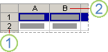
2. Column heading
You can also select cells in a row or column by selecting the first cell and then pressing CTRL+SHIFT+ARROW key (RIGHT ARROW or LEFT ARROW for rows, UP ARROW or DOWN ARROW for columns).
Note: If the row or column contains data, CTRL+SHIFT+ARROW key selects the row or column to the last used cell. Pressing CTRL+SHIFT+ARROW key a second time selects the entire row or column.
Adjacent rows or columns
Drag across the row or column headings. Or select the first row or column; then hold down SHIFT while you select the last row or column.
Nonadjacent rows or columns
Click the column or row heading of the first row or column in your selection; then hold down CTRL while you click the column or row headings of other rows or columns that you want to add to the selection.
The first or last cell in a row or column
Select a cell in the row or column, and then press CTRL+ARROW key (RIGHT ARROW or LEFT ARROW for rows, UP ARROW or DOWN ARROW for columns).
The first or last cell on a worksheet or in a Microsoft Office Excel table
Press CTRL+HOME to select the first cell on the worksheet or in an Excel list.
Press CTRL+END to select the last cell on the worksheet or in an Excel list that contains data or formatting.
Cells to the last used cell on the worksheet (lower-right corner)
Select the first cell, and then press CTRL+SHIFT+END to extend the selection of cells to the last used cell on the worksheet (lower-right corner).
Cells to the beginning of the worksheet
Select the first cell, and then press CTRL+SHIFT+HOME to extend the selection of cells to the beginning of the worksheet.
More or fewer cells than the active selection
Hold down SHIFT while you click the last cell that you want to include in the new selection. The rectangular range between the active cell and the cell that you click becomes the new selection.
Need more help?
You can always ask an expert in the Excel Tech Community or get support in the Answers community.
Источник
How to select cells/ranges by using Visual Basic procedures in Excel
Microsoft provides programming examples for illustration only, without warranty either expressed or implied. This includes, but is not limited to, the implied warranties of merchantability or fitness for a particular purpose. This article assumes that you are familiar with the programming language that is being demonstrated and with the tools that are used to create and to debug procedures. Microsoft support engineers can help explain the functionality of a particular procedure, but they will not modify these examples to provide added functionality or construct procedures to meet your specific requirements. The examples in this article use the Visual Basic methods listed in the following table.
The examples in this article use the properties in the following table.
How to Select a Cell on the Active Worksheet
To select cell D5 on the active worksheet, you can use either of the following examples:
How to Select a Cell on Another Worksheet in the Same Workbook
To select cell E6 on another worksheet in the same workbook, you can use either of the following examples:
Or, you can activate the worksheet, and then use method 1 above to select the cell:
How to Select a Cell on a Worksheet in a Different Workbook
To select cell F7 on a worksheet in a different workbook, you can use either of the following examples:
Or, you can activate the worksheet, and then use method 1 above to select the cell:
How to Select a Range of Cells on the Active Worksheet
To select the range C2:D10 on the active worksheet, you can use any of the following examples:
How to Select a Range of Cells on Another Worksheet in the Same Workbook
To select the range D3:E11 on another worksheet in the same workbook, you can use either of the following examples:
Or, you can activate the worksheet, and then use method 4 above to select the range:
How to Select a Range of Cells on a Worksheet in a Different Workbook
To select the range E4:F12 on a worksheet in a different workbook, you can use either of the following examples:
Or, you can activate the worksheet, and then use method 4 above to select the range:
How to Select a Named Range on the Active Worksheet
To select the named range «Test» on the active worksheet, you can use either of the following examples:
How to Select a Named Range on Another Worksheet in the Same Workbook
To select the named range «Test» on another worksheet in the same workbook, you can use the following example:
Or, you can activate the worksheet, and then use method 7 above to select the named range:
How to Select a Named Range on a Worksheet in a Different Workbook
To select the named range «Test» on a worksheet in a different workbook, you can use the following example:
Or, you can activate the worksheet, and then use method 7 above to select the named range:
How to Select a Cell Relative to the Active Cell
To select a cell that is five rows below and four columns to the left of the active cell, you can use the following example:
To select a cell that is two rows above and three columns to the right of the active cell, you can use the following example:
An error will occur if you try to select a cell that is «off the worksheet.» The first example shown above will return an error if the active cell is in columns A through D, since moving four columns to the left would take the active cell to an invalid cell address.
How to Select a Cell Relative to Another (Not the Active) Cell
To select a cell that is five rows below and four columns to the right of cell C7, you can use either of the following examples:
How to Select a Range of Cells Offset from a Specified Range
To select a range of cells that is the same size as the named range «Test» but that is shifted four rows down and three columns to the right, you can use the following example:
If the named range is on another (not the active) worksheet, activate that worksheet first, and then select the range using the following example:
How to Select a Specified Range and Resize the Selection
To select the named range «Database» and then extend the selection by five rows, you can use the following example:
How to Select a Specified Range, Offset It, and Then Resize It
To select a range four rows below and three columns to the right of the named range «Database» and include two rows and one column more than the named range, you can use the following example:
How to Select the Union of Two or More Specified Ranges
To select the union (that is, the combined area) of the two named ranges «Test» and «Sample,» you can use the following example:
that both ranges must be on the same worksheet for this example to work. Note also that the Union method does not work across sheets. For example, this line works fine.
returns the error message:
Union method of application class failed
How to Select the Intersection of Two or More Specified Ranges
To select the intersection of the two named ranges «Test» and «Sample,» you can use the following example:
Note that both ranges must be on the same worksheet for this example to work.
Examples 17-21 in this article refer to the following sample set of data. Each example states the range of cells in the sample data that would be selected.
How to Select the Last Cell of a Column of Contiguous Data
To select the last cell in a contiguous column, use the following example:
When this code is used with the sample table, cell A4 will be selected.
How to Select the Blank Cell at Bottom of a Column of Contiguous Data
To select the cell below a range of contiguous cells, use the following example:
When this code is used with the sample table, cell A5 will be selected.
How to Select an Entire Range of Contiguous Cells in a Column
To select a range of contiguous cells in a column, use one of the following examples:
When this code is used with the sample table, cells A1 through A4 will be selected.
How to Select an Entire Range of Non-Contiguous Cells in a Column
To select a range of cells that are non-contiguous, use one of the following examples:
When this code is used with the sample table, it will select cells A1 through A6.
How to Select a Rectangular Range of Cells
In order to select a rectangular range of cells around a cell, use the CurrentRegion method. The range selected by the CurrentRegion method is an area bounded by any combination of blank rows and blank columns. The following is an example of how to use the CurrentRegion method:
This code will select cells A1 through C4. Other examples to select the same range of cells are listed below:
In some instances, you may want to select cells A1 through C6. In this example, the CurrentRegion method will not work because of the blank line on Row 5. The following examples will select all of the cells:
How to Select Multiple Non-Contiguous Columns of Varying Length
To select multiple non-contiguous columns of varying length, use the following sample table and macro example:
When this code is used with the sample table, cells A1:A3 and C1:C6 will be selected.
Notes on the examples
The ActiveSheet property can usually be omitted, because it is implied if a specific sheet is not named. For example, instead of
The ActiveWorkbook property can also usually be omitted. Unless a specific workbook is named, the active workbook is implied.
When you use the Application.Goto method, if you want to use two Cells methods within the Range method when the specified range is on another (not the active) worksheet, you must include the Sheets object each time. For example:
For any item in quotation marks (for example, the named range «Test»), you can also use a variable whose value is a text string. For example, instead of
Источник
Select rows and columns in an Excel table
You can select cells and ranges in a table just like you would select them in a worksheet, but selecting table rows and columns is different from selecting worksheet rows and columns.
A table column with or without table headers
Click the top edge of the column header or the column in the table. The following selection arrow appears to indicate that clicking selects the column.

Note: Clicking the top edge once selects the table column data; clicking it twice selects the entire table column.
You can also click anywhere in the table column, and then press CTRL+SPACEBAR, or you can click the first cell in the table column, and then press CTRL+SHIFT+DOWN ARROW.
Note: Pressing CTRL+SPACEBAR once selects the table column data; pressing CTRL+SPACEBAR twice selects the entire table column.
Click the left border of the table row. The following selection arrow appears to indicate that clicking selects the row.

You can click the first cell in the table row, and then press CTRL+SHIFT+RIGHT ARROW.
All table rows and columns
Click the upper-left corner of the table. The following selection arrow appears to indicate that clicking selects the table data in the entire table.

Click the upper-left corner of the table twice to select the entire table, including the table headers.
You can also click anywhere in the table, and then press CTRL+A to select the table data in the entire table, or you can click the top-left most cell in the table, and then press CTRL+SHIFT+END.
Press CTRL+A twice to select the entire table, including the table headers.
Need more help?
You can always ask an expert in the Excel Tech Community or get support in the Answers community.
Источник
Select cell contents in Excel
In Excel, you can select cell contents of one or more cells, rows and columns.
Note: If a worksheet has been protected, you might not be able to select cells or their contents on a worksheet.
Select one or more cells
-
Click on a cell to select it. Or use the keyboard to navigate to it and select it.
-
To select a range, select a cell, then with the left mouse button pressed, drag over the other cells.
Or use the Shift + arrow keys to select the range.
-
To select non-adjacent cells and cell ranges, hold Ctrl and select the cells.
Select one or more rows and columns
-
Select the letter at the top to select the entire column. Or click on any cell in the column and then press Ctrl + Space.
-
Select the row number to select the entire row. Or click on any cell in the row and then press Shift + Space.
-
To select non-adjacent rows or columns, hold Ctrl and select the row or column numbers.
Select table, list or worksheet
-
To select a list or table, select a cell in the list or table and press Ctrl + A.
-
To select the entire worksheet, click the Select All button at the top left corner.

Note: In some cases, selecting a cell may result in the selection of multiple adjacent cells as well. For tips on how to resolve this issue, see this post How do I stop Excel from highlighting two cells at once? in the community.
|
To select |
Do this |
|---|---|
|
A single cell |
Click the cell, or press the arrow keys to move to the cell. |
|
A range of cells |
Click the first cell in the range, and then drag to the last cell, or hold down SHIFT while you press the arrow keys to extend the selection. You can also select the first cell in the range, and then press F8 to extend the selection by using the arrow keys. To stop extending the selection, press F8 again. |
|
A large range of cells |
Click the first cell in the range, and then hold down SHIFT while you click the last cell in the range. You can scroll to make the last cell visible. |
|
All cells on a worksheet |
Click the Select All button.
To select the entire worksheet, you can also press CTRL+A. Note: If the worksheet contains data, CTRL+A selects the current region. Pressing CTRL+A a second time selects the entire worksheet. |
|
Nonadjacent cells or cell ranges |
Select the first cell or range of cells, and then hold down CTRL while you select the other cells or ranges. You can also select the first cell or range of cells, and then press SHIFT+F8 to add another nonadjacent cell or range to the selection. To stop adding cells or ranges to the selection, press SHIFT+F8 again. Note: You cannot cancel the selection of a cell or range of cells in a nonadjacent selection without canceling the entire selection. |
|
An entire row or column |
Click the row or column heading.
1. Row heading 2. Column heading You can also select cells in a row or column by selecting the first cell and then pressing CTRL+SHIFT+ARROW key (RIGHT ARROW or LEFT ARROW for rows, UP ARROW or DOWN ARROW for columns). Note: If the row or column contains data, CTRL+SHIFT+ARROW key selects the row or column to the last used cell. Pressing CTRL+SHIFT+ARROW key a second time selects the entire row or column. |
|
Adjacent rows or columns |
Drag across the row or column headings. Or select the first row or column; then hold down SHIFT while you select the last row or column. |
|
Nonadjacent rows or columns |
Click the column or row heading of the first row or column in your selection; then hold down CTRL while you click the column or row headings of other rows or columns that you want to add to the selection. |
|
The first or last cell in a row or column |
Select a cell in the row or column, and then press CTRL+ARROW key (RIGHT ARROW or LEFT ARROW for rows, UP ARROW or DOWN ARROW for columns). |
|
The first or last cell on a worksheet or in a Microsoft Office Excel table |
Press CTRL+HOME to select the first cell on the worksheet or in an Excel list. Press CTRL+END to select the last cell on the worksheet or in an Excel list that contains data or formatting. |
|
Cells to the last used cell on the worksheet (lower-right corner) |
Select the first cell, and then press CTRL+SHIFT+END to extend the selection of cells to the last used cell on the worksheet (lower-right corner). |
|
Cells to the beginning of the worksheet |
Select the first cell, and then press CTRL+SHIFT+HOME to extend the selection of cells to the beginning of the worksheet. |
|
More or fewer cells than the active selection |
Hold down SHIFT while you click the last cell that you want to include in the new selection. The rectangular range between the active cell and the cell that you click becomes the new selection. |
Need more help?
You can always ask an expert in the Excel Tech Community or get support in the Answers community.
See Also
Select specific cells or ranges
Add or remove table rows and columns in an Excel table
Move or copy rows and columns
Transpose (rotate) data from rows to columns or vice versa
Freeze panes to lock rows and columns
Lock or unlock specific areas of a protected worksheet
Need more help?
Want more options?
Explore subscription benefits, browse training courses, learn how to secure your device, and more.
Communities help you ask and answer questions, give feedback, and hear from experts with rich knowledge.
Data Analysis Tool
Real Statistics Data Analysis Tool: The Extract Columns from Data Range data analysis tool supplied by the Real Statistics Resource Pack enables you to select a subset of columns from a data range. It is especially useful when data for only certain random variables are to be used in a particular analysis. The use of this tool is illustrated in Example 1.
Example 1: Extract the Poverty, Infant Mort, Doctors, Traf Deaths, and Income columns from the data range A3:J22 in Figure 1.
Figure 1 – Extract Columns from Data Range dialog box
Initial dialog box
Press Ctrl-m and choose the Extract Columns from Data Range option (from the Desc tab or the main menu if using the original user interface). Fill in the dialog box that appears with the Input Range and Output Range as shown in Figure 1, and then click on the OK button. You can ignore the Code type and Degree options for now.
Note that the data in the Input Range must contain unique column headings.
Revised dialog box
The dialog box will now change as shown on the right side of Figure 2. Highlight the first three columns on the list by clicking on State and then, while pressing down on the Shift key down, click on Infant Mort. Next, press the Add Column button. The State, Poverty, and Infant Mort columns are now copied to the output as shown.
Figure 2 – Copy Columns from a Data Range
You can copy the remaining columns of interest by clicking on Doctors, Traf Deaths, and Income in the list while holding down the Ctrl key and then pressing the Add Column button. Finally, click on the Done button to close the dialog box. The result is shown in Figure 3.
The Add Code, Add Inter, and Add Power buttons are explained on the following web pages:
- Add Code: Categorical Coding for Regression
- Add Inter: Interaction
- Add Power: Polynomial Regression Analysis Tool
Looking at the data
If while performing any of these steps, you need to look at the Excel workbook, you can simply click on the Data button on the lower right-hand side of the dialog box. You are advised not to change anything in the workbook when you do this.
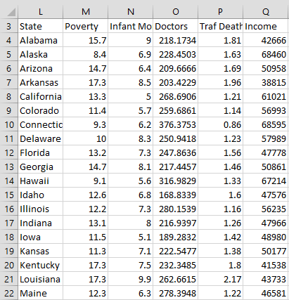
Figure 3 – Output from Extract Columns data analysis tool
Worksheet Function
Real Statistics Function: You can also use the following array function from the Real Statistics Resource Pack to select columns from an array or data range.
SelectCols(R1, selections) – returns an array with the columns from R1 specified in the string selections in the order in which they appear. selections specifies a list of column indices separated by commas. Not all columns in R1 need to be included in the output, some columns can be included multiple times, and the order of the columns can be different from how they appear in R1.
SelectCols(R1, selections, sortcol) – returns an array with the columns from R1 as specified for SelectCols(R1, selections) except that the rows in the output are sorted based on the elements in the sortcolth column of the output, in a fashion similar to the Real Statistics function QSORTRows.
If, for example, R1 is a 4 × 5 array, then selections could take the form “2, 3, 2”. The output from SelectCols(R1, “2,3,2”) would then consist of the 2nd, 3rd, and 2nd columns of R1 in that order where the 2nd column appears twice. In this case, SelectCols(R1, “2,3,2”, 2) would yield the same output in sorted order based on the elements in the 2nd column of the output (which is the 3rd column of R1).
Note that SelectCols plays a similar role to the Excel 365 function CHOOSECOLS (see Excel Reformatting Functions).
Using this worksheet function
Example 2: Create a new range consisting of the 2nd, 3rd, and 1st columns of the data in range A3:D14 of Figure 3. Also create a new range which changes the order of the columns of the data in range A3:D14 to the 3rd, 2nd, 1st, and 4th columns in that order and sorts the rows of this new range based on the 3rd column of A3:D14 (i.e. the 1st column of the new range).
The first of these ranges is shown in range F3:H14 of Figure 4 and is calculated by the array formula =SelectCols(A3:D14,”2,3,1”). The second is shown in range J3:M14 and is calculated by the array formula =SelectCols(A3:D14,”3,2,1,4”,1).
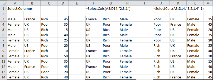
Figure 4 – Selecting columns from a data range
Examples Workbook
Click here to download the Excel workbook with the examples described on this webpage.
References
Howell, D. C. (2010) Statistical methods for psychology (7th ed.). Wadsworth, Cengage Learning.
https://labs.la.utexas.edu/gilden/files/2016/05/Statistics-Text.pdf
I would like to get a range of the first column from a larger range. For example:
If the range is $E$9:$I$259, the result should be $E$9:$E259
How can I achieve this?
![]()
jordanz
3414 silver badges11 bronze badges
asked Apr 12, 2013 at 14:45
![]()
NCCNCC
81912 gold badges25 silver badges43 bronze badges
0
1 Answer
By using the columns collection of the range object like so:
Range("$E$9:$I$259").Columns(1)
![]()
JvdV
66.6k8 gold badges38 silver badges68 bronze badges
answered Apr 12, 2013 at 14:52
![]()
Dave SextonDave Sexton
10.6k3 gold badges42 silver badges55 bronze badges
4