
This tutorial talks about how to select cells with formula in Excel. In tutorial below I have compiled various methods to do the same. And the best part is that most the methods can select cells with formula without using any other third party software. I have also added a plugin in the following list to select cells in Excel that contain specific formula.
Selecting cells that contain formula or specific formula can be useful in many cases. Let’s say, you have an Excel sheet that has tons of cells in it with various formulas and you want to delete or change those cells. Doing it manually will take a fair amount of time. That’s where this tutorial comes in handy. In this tutorial I will explain how to select cells with formula in Excel.
You may already know how to select and count cells by background or font color. In the same way you can also select cells with formula in Excel with the help of the following methods. Let’s see how.
Do note that there could be various scenarios of selecting cells with formaula in Excel. You might want to simply select all the cells that have any formula, or you might want to select only those cells that have a spefic formula. I have explained all these scenarios here. If you have a selection scenario that I missed to cover here, do let me know in comments, and I will try to find a way for that as well.
This is the most basic scenario in which you want to simply select all the cells in a worksheet or selection that contain a formula. I will use the “Go to Special” tool of Excel to do the same. This Excel tool lets you select all the cells that have formula in them. Also, using the same tool, you can also select cells based on what is the output of formula in them. For example, you can choose to select only those cells in which formula would always product a numeric output (like, Sum, Avg, etc.).
To select cells that contain a formula, follow these simple steps.
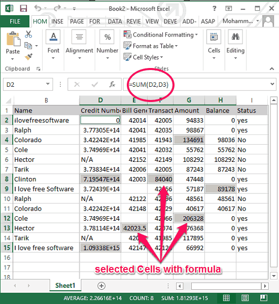
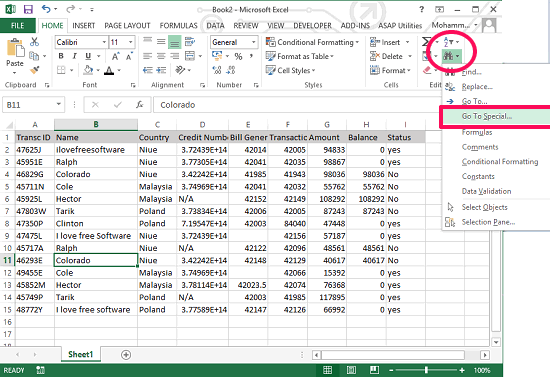
Step 1: Open your Excel sheet in which you want to select the cells that have formula. And invoke Go to Special Tool from the Home ribbon.
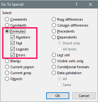
Step 2: From the Go To Special tool’s interface, check the Formula option and you can also filter the result by specifying the output type of the formula.
Step 3: To select all the cells containing a formula, hit the OK button. After that you will see all the cells that have formula have been selected.
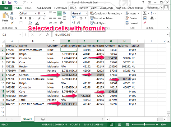
This is the fastest and easiest way to select cells with formula in Excel. And after you have your selected cells, you can do whatever you want to do with them.
How to Select Cells That Have a Specific Formula in Excel
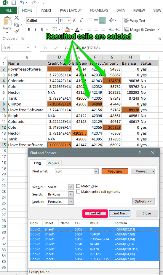
Let’s say you don’t want to select all the cells that have a formula, but only want to select those cells that have a specific formula. That is possible as well. You would be surprised to know that “Find” tool of the Excel will do it for you. The Find tool of Excel is very powerful. This tool can not only find the value, but also list all the cells that contain the specified formula text. And after that you can do whatever you want with the selected cells.
Follow these simple steps to select cells in Excel that contain a specific formula:
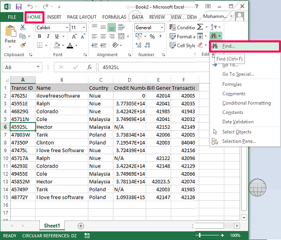
Step 1: Open any Excel sheet that contains cells with formula that you want to select. And click on the Find tool from the end of the Home tab of Excel. Or just to Ctrl+F.
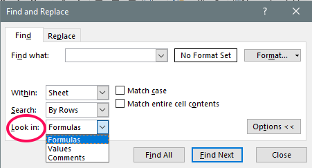
Step 2: Now, Expand the interface of the Find tool by clicking on the Options button. After that, navigate to “Look in” drop down and select “Formulas” from it.
Step 3: Type the formula text in the “Find What” text box, and hit Find All button. You will see that it will list all the cells that contain that formula text.
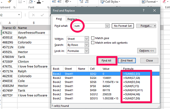
Now, if you want to select all the cells, click on any empty space in the result cells list and press Ctrl+A keyboard shortcut. After that, all the cells will get selected and you may now close the Find tool.
So, in this way you can easily select cells in Excel that contain a specific formula.
How to Select Cells With Formula in Excel that have a Specific font or font color
Let’s say you have a crazy scenario that you want to select all the cells in Excel that have a formula, and also they have a specific font, or a specific font color. I am not sure why you would run in this type of scenario, but in case you do, worry not. Here I have provided a solution for that too.
In this method I will use some filters along with the Find tool of Excel. After searching a specific formula text, the method will list all the cells that have the specified font or font color.
Here is how to do this:
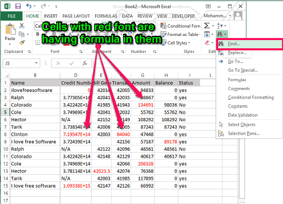
Step 1: Open up any worksheet that contains some formatted cells and also have formulas in them. Open Find tool from the Home ribbon.
Step 2: Now, Expand the interface of the Find & Select tool by clicking on the Options button. After that, navigate to “Look in” drop down and select “Formulas” from it.
Step 3: Click on Format button and a window will pop up with various tabs it. Navigate to the Fonts tab and specify the font type there. For saving time, you can also directly specify font formatting from an existing cell from your sheet. To do this use the Choose Format From Cell button and specify the cell by selecting it from your Excel sheet.
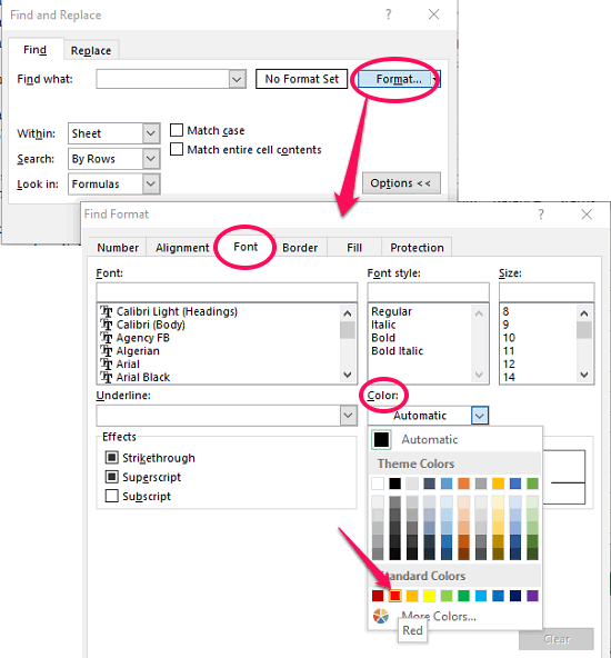
Step 4: Type the formula text in the Find What text box, and hit Find All button. You will see that it will list all the cells that contain that formula text and has the font formatting that you selected.
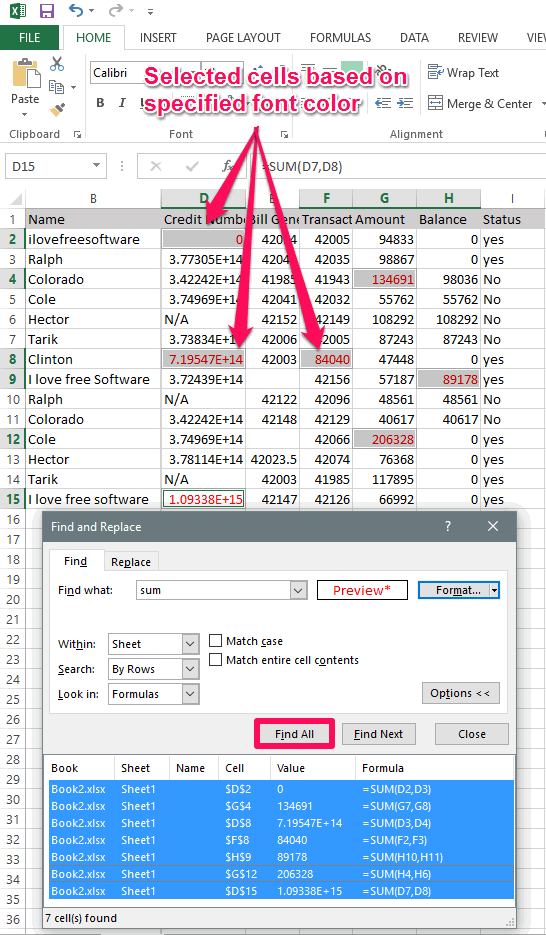
Now, if you want to select all the cells then click on any empty space in the result window and press the Ctrl+A keyboard shortcut. After that, all the cells will get selected and you may now close the Find & Select tool.
So, in this way you can select all the cells that contain a specific formula and font formatting. And you can do it in seconds.
Now, what if you want to select all the cells that had any formula, but have a specific formatting. For that, you can use Asap Utilities, that I have covered at the end of this tutorial.
Method 4: Select Cells With Formula in Excel That Have a Specific Background color
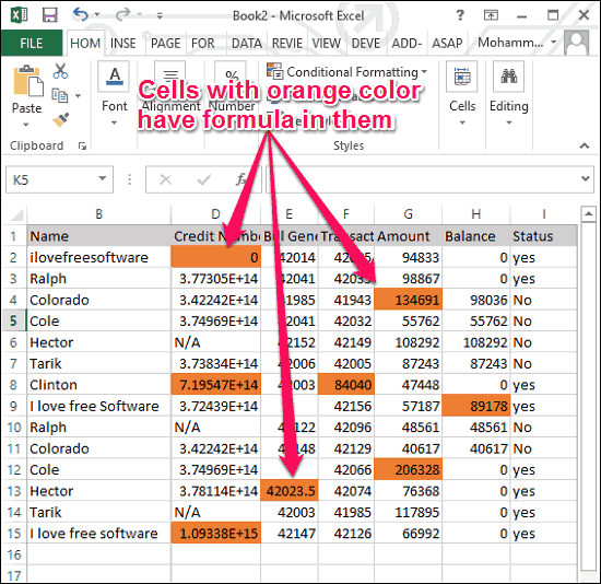
In the previous method I have explained how to select cells that contain specific formula and font. Now, in a similar way I will show how to select cells in Excel that have a specific formula and a specific background color. Let’s see how.
Step 1: Open an Excel sheet that has some colored cells with formulas in it. Invoke the Find tool using the keyboard shortcut Ctrl+F.
Step 2: After expanding the interface of the Find tool, configure it to search text in formulas as I have explained in above methods.
Step 3: Click on Format button and a window will pop up. Navigate to the Fill tab and specify the background color there. You can also directly specify the fill color from an existing cell of your sheet. To do this use the Choose Format From Cell button and specify the reference cell by selecting it from your Excel sheet.
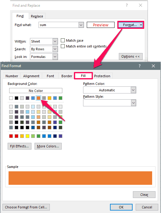
Step 4: Type the formula text in the Find What text box, and hit Find All button. You will see that it will list all the cells that contain that formula text and background color.
If you want to select all the cells, then click on any empty space in the result window and press the Ctrl+A keyboard shortcut. After that, all the cells will get selected and you can now close the Find tool.
So, in this way, you can select cells with formula in Excel and with the specified background color.
Bonus: Select Cells with Formula in Excel via Plugin
In the above mentioned methods I have explained how to select cells with formula in Excel and with the various formatting options. And for them I used built in functions of Excel. Now, in this section I will show you how you can do the same using an Excel plugin.
Asap Utilities package for Excel comes with tons of features to manipulate excel data that is difficult to do using the built in functions of Excel. However, it is only free for educational use.
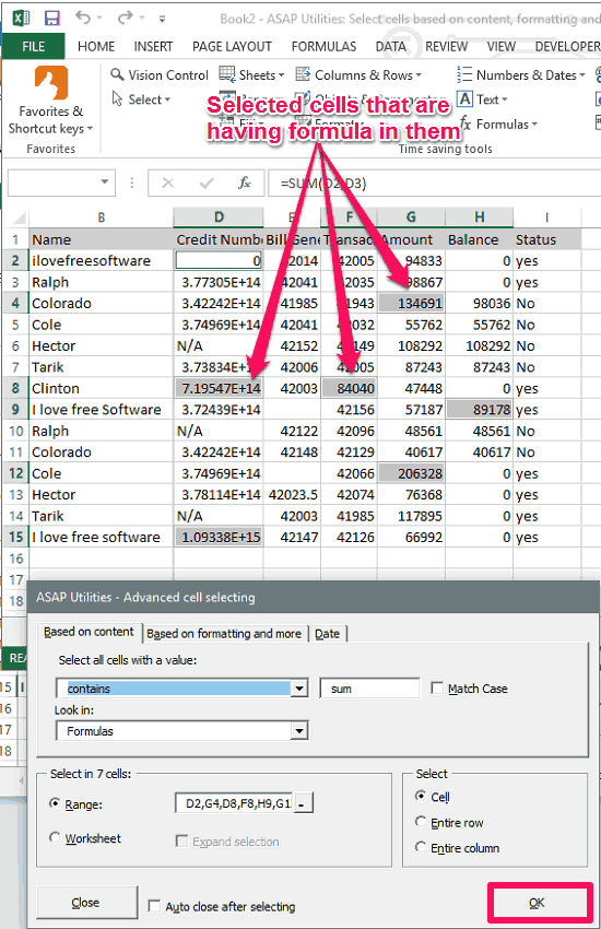
One of the modules in the Asap Utilities package is Selecting cells based on content, formatting and more. I will use this tool of Asap Utilities to do the same. To see how to do it, simply follow these steps.
Step 1: Download and install Asap Utilities using this link. After installing it, you will see that it adds an additional tab in the Excel window
.Step 2: Open up any Excel sheet and navigate to the Asap Utilities tab and click on the Select drop down.
Step 3: Choose Selecting cells based on content, formatting and more option from the list and a window will pop up. And, you will have to configure various options there.
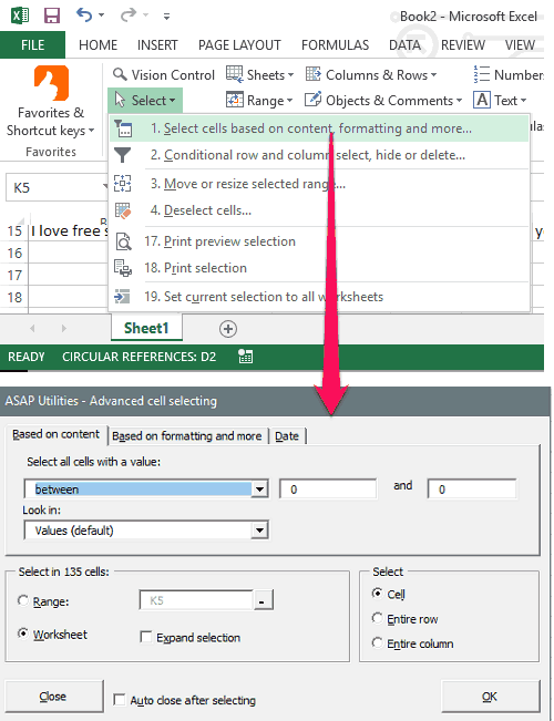
Step 4: Go to the first tab “Based on Content”. In this, choose “contains” from the first drop-down. And in the “Look in” drop down, choose “Formulas”.

Step 5: Type the name of the formula to be searched and hit the OK button.
At the end of the step 5, you will see that all the cells will get selected that meet with the specified condition.
So, it was the other nice way to select cells in Excel. If you are a plugin enthusiast, then you may give this method a try.
Also, if you want to select all cells that have a formula and have a specific formatting, then leave the drop-down next to “contains” blank. Then head over to “Based on formatting and more” and specify the formatting that you wish to select. In this way you will be able to select cells with formula and specific formatting.
Closing Thoughts
In the tutorial above, I have demonstrated various methods to select cells with formula in Excel. I have also explained to achieve the same with various criteria. So, if you are looking for the ways to do the same, then this tutorial should help you. Depending on what suits you need, you can give a try to any of the mentioned methods.
To select the cells which contain only formulas, we can use the Go-To option in Microsoft Excel.
Go To Special: — This option is used to quickly re-direct to different cells in Excel.
Shortcut keys: F5 and Ctrl+G
Command button: Go to the Home tab>Select Find & Select >Select Go to Special
Let’s take an example to understand how we can select the cells which contain formulas.
We have a sales report, in which some cells contain formula. We need to select these cells.
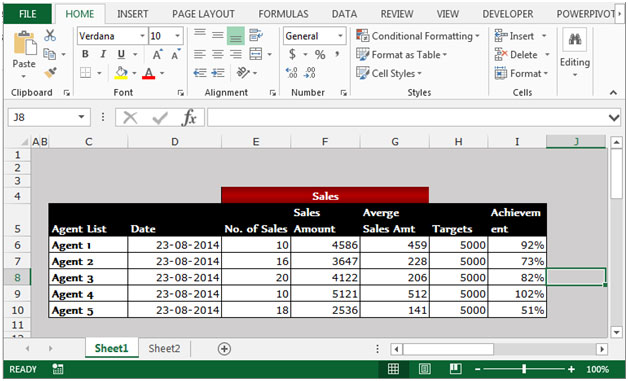
To Select the cells which contain formulas, follow the below given steps:-
- Go to the Home tab.
- Click on Find & Select from the Editing group.
- The Find & Select drop down menu will appear.
- Click on Formulas from the drop down menu.

- All cells containing formulas will get selected.
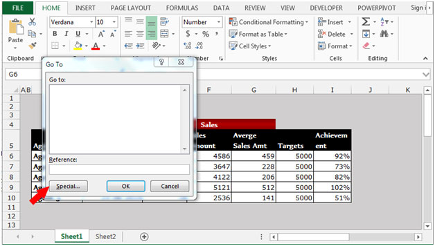
- In the Home tab from the editing group, click on Find & Select and select Go To Special or you can press the shortcut key F5.
- When we press the F5 key, the Go-to dialog box will appear.
- Click on Special button in the bottom left corner.
- The Go-to-Special dialog box will open.
- Select the Formulas option.
- Click on OK.
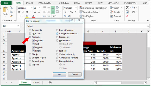
All type of formulas will get selected -numbers, text, logical, and errors in your workbook.
By using this method, we can identify that which cells contain the formulas and also highlight them.
![]()
If you liked our blogs, share it with your friends on Facebook. And also you can follow us on Twitter and Facebook.
We would love to hear from you, do let us know how we can improve, complement or innovate our work and make it better for you. Write us at info@exceltip.com
A few days back I had a huge spreadsheet in which I had to find out the cells containing formulas. Initially, I was totally clueless about how this task can be done.
But later after doing some Google searches, I got a few ideas on how I can effortlessly identify the formula cells in excel.
And today to share my experiences with you guys, In this post I will throw some light on a few methods that can help you to find out formula cells in your spreadsheets.
So here we go:
Method 1: Using ‘Go To Special’ Option:
In Excel ‘Go To Special’ is a very handy option when it comes to finding the cells with formulas. ‘Go to Special’ option has a radio button “Formulas” and selecting this radio button enables it to select all the cells containing formulas.
Later you can change the formatting or background color of the selected cells to make them stand out from the rest. Below is the step by step instructions for accomplishing this:
1. With your excel sheet opened navigate to the ‘Home’ tab > ‘Find & Select’ > ‘Go To Special’. Alternatively, you can also press ‘F5’ and then ‘Alt + S’ to open the ‘Go to Special’ dialog.

2. Next, in the ‘Go to Special’ window select the ‘Formulas’ radio button. After checking this radio button you will notice that few checkboxes (like Numbers, Errors, Logical, and Text) are enabled, these checkboxes signify the return type of the formulas.
So, if you select the ‘Formulas’ radio button and only check the ‘Numbers’ checkbox then it will just search the Formulas whose return type is a number. Here in our example, we will keep all of these return types checked.
3. After this click the ‘Ok’ button and all the cells that contain formulas get selected.
4. Next, without clicking anywhere on your spreadsheet change the background color of all the selected cells.
5. Now your formula cells can be easily identified.
Method 2: Using a built-in Excel formula
If you have worked with excel formulas then probably you may be knowing that excel has a formula that can find whether a cell contains a formula or not. The formula that I am talking about is:
=ISFORMULA(reference)
Here ‘reference’ signifies the cell position which you wish to check for the presence of a formula.
For example: If you wish to check the cell ‘A2’ for the existence of a formula then you can use this function as
=ISFORMULA(A2)
This function results in a Boolean output i.e. True or False. True signifies that the cell contains formulas while False tells that cell doesn’t contain any formulas.
Method 3: Using a Macro for identifying the cells that contain formulas:
I have created a VBA Macro that can find and color any cells that contain the formula in the total used range of the Active sheet. To use this macro simply follow the below procedure:
1. Open your spreadsheet and hit the ‘Alt + F11’ keys to open the VBA editor.

2. Next, navigate to ‘Insert‘ > ‘Module‘ and then paste the below macro in the editor.
Sub FindFormulaCells()
For Each cl In ActiveSheet.UsedRange
If cl.HasFormula() = True Then
cl.Interior.ColorIndex = 24
End If
Next cl
End Sub
3. For running this formula press the “F5” key.
4. This Macro will change the background colour of all the formula containing cells and thus makes it easier to identify them easily.
Recommended Reading: How to add a Checkbox in excel
Find | Replace | Go To Special
You can use Excel’s Find and Replace feature to quickly find specific text and replace it with other text. You can use Excel’s Go To Special feature to quickly select all cells with formulas, notes, conditional formatting, constants, data validation, etc.
Find
To quickly find specific text, execute the following steps.
1. On the Home tab, in the Editing group, click Find & Select.

2. Click Find.

The ‘Find and Replace’ dialog box appears.
3. Type the text you want to find. For example, type Ferrari.
4. Click ‘Find Next’.

Excel selects the first occurrence.

5. Click ‘Find Next’ to select the second occurrence.

6. To get a list of all the occurrences, click ‘Find All’.

Replace
To quickly find specific text and replace it with other text, execute the following steps.
1. On the Home tab, in the Editing group, click Find & Select.
2. Click Replace.

The ‘Find and Replace’ dialog box appears (with the Replace tab selected).
3. Type the text you want to find (Veneno) and replace it with (Diablo).
4. Click ‘Find Next’.

Excel selects the first occurrence. No replacement has been made yet.

5. Click ‘Replace’ to make a single replacement.

Note: use ‘Replace All’ to replace all occurrences.
Go To Special
You can use Excel’s Go To Special feature to quickly select all cells with formulas, notes, conditional formatting, constants, data validation, etc. For example, to select all cells with formulas, execute the following steps.
1. Select a single cell.
2. On the Home tab, in the Editing group, click Find & Select.
3. Click Go To Special.

Note: Formulas, Notes, Conditional formatting, Constants and Data Validation are shortcuts. They can also be found under Go To Special.
4. Select Formulas and click OK.

Note: you can search for cells with formulas that return Numbers, Text, Logicals (TRUE and FALSE) and Errors. These check boxes are also available if you select Constants.
Excel selects all cells with formulas.

General note: if you select a single cell before you click Find, Replace or Go To Special, Excel searches the entire worksheet. To search a range of cells, first select a range of cells.
The Excel Formulas Ultimate Guide
Introduction to Excel Formulas
In this guide, we are going to cover everything you need to know about Excel Formulas. Learning how to create a formula in Excel is the building block to the exciting journey to become an Excel Expert. So, let’s get started!
What is an Excel Formula?
Excel Formulas are often referred to as Excel Functions and it’s no big deal but there is a difference, a function is a piece of code that executes a predefined calculation, and a formula is an equation created by the user.
A formula is an expression that operates on values in a cell or range of cells. An example of a formula looks like this: = A2 + A3 + A4 + A5. This formula will result in the sum of the range of values from cell A2 to cell A5.
A function is a predetermined formula in Excel. It shows calculations in a particular order defined by its parameters. An example of a function is =SUM (A2, A5). This function will also provide the addition of values in the range of cells from A2 to A5 but here instead of specifying each cell address we are using the SUM function.
How To Write Excel Formulas
Let’s look at how to write a formula on MS Excel. To begin with, a formula always starts with a ‘+’ or ‘=’ sign, if you start writing the formula without any of these two signs, Excel will treat the value in that cell as text and will not perform any function.
In the screenshot below, you need to calculate the total sales amount by multiplying quantity sold with unit price. Select cell D2, type the formula ‘=B2*C2’ and press Enter. The result will display on cell D2.

Apply A Formula To An Entire Column Or Range
To copy a formula to adjacent cells, you can do the following:
- Select the cell with the formula and the adjacent cells you want to fill, then drag the fill handle.

- Select the cell with the formula and the adjacent cells you want to fill, then press Ctrl+D to fill the formula down in a column, or Ctrl+R to fill the formula to the right in a row.
- Select the cell with the formula and the adjacent cells you want to fill, then Click Home > Fill, and choose either Down, Right, Up, or Left.

How to Copy A Formula And Paste It
Excel allows you to copy the formula entered in a cell and paste it on to another cell, which can save both time and effort. To copy paste a formula:
- Select the cell whose formula you wish to copy
- Press Ctrl + C to copy the content
- Select the cell or cells where you wish to paste the formula. The copied cells will now have a dashed box around them.
- Press Alt + E + S to open the paste special box and select ‘Formula’ or Press “F’ to paste the formula.

- The formula will be pasted into the selected cells.
Basic Excel Formulas
Let’s start off with simple Excel Formulas. In the screenshot below, there are two columns containing numbers and we would like to use different operators like addition, subtraction, multiplication, and division on those to get different results. Excel uses standard operators for formulas, such as a plus sign for addition (+), a minus sign for subtraction (-), an asterisk for multiplication (*), a forward slash for division (/).

- Addition– To add values in the two columns, simply type the formula =A2+B2 on cell C2 and then copy paste the same on the cells below.
- Subtraction – To subtract values in Column B from Column A, simply type the formula =B2-A2 on cell C2 and then copy paste the same on the cells below.
- Multiplication – To multiply values in the two columns, simply type the formula =A2*B2 on cell C2 and then copy paste the same on the cells below.
- Division – To divide values in Column a by values in Column B, simply type the formula =A2/B2 on cell C2 and then copy paste the same on the cells below.
We can also calculate the percentage using Excel Formulas. In the image below, we have sales in Year 1 and Year 2 and we would like to know the % growth in sales from Year 1 to Year 2.

To do that, select cell C2 and type the formula = (B2 – A2)/B2*100
Basic Excel Functions
A function is a predefined formula that performs calculations using specific values in a particular order. Excel includes many common functions that can be useful for quickly finding the sum, average, count, maximum value, and minimum value for a range of cells. a function must be written a specific way, which is called the syntax.
The basic syntax for a function is an equals sign (=), the function name, and one or more arguments. A Function is generally comprised of two components:
1) A function name -The name of a function indicates the type of math Excel will perform.
2) An argument – It is the values that a function uses to perform operations or calculations. The type of argument a function uses is specific to the function. Common arguments that are used within functions include numbers, text, cell references, and names
Let’s look at some common Excel Functions:
SUM Function
The SUM formula adds 2 or more numbers together. You can use cell references as well in this formula.
Syntax: =SUM(number1, [number2], …)
Example: =SUM(A2:A8) or SUM(A2:A7, A9, A12:A15)

AUTOSUM Function
The AutoSum command allows you to automatically insert the most common functions into your formula, including SUM, AVERAGE, COUNT, MIN, and MAX.
Select the cell where you want the formula, Go to Home > Click on AutoSum > From the dropdown click on “Sum” > Enter.

COUNT Function
If you wish to how many cells are there in a selected range containing numeric values, you can use the function COUNT. It will only count cells that contain either numbers or dates.
Syntax: =COUNT(value1, [value2], …)
In the example below, you can see that the function skips cell A6 (as it is empty) and cell A11 (as it contains text) and gives you the output 9.
COUNTA Function
Counts the number of non-empty cells in a range. It will include cells that have any character in them and only exclude blank cells.
Syntax: =COUNTA(value1, [value2], …)
In the example below, you can see that only cell A6 is not included, all other 10 cells are
counted.

AVERAGE Function
This function calculates the average of all the values or range of cells included in the parentheses.
Syntax: =AVERAGE(value1, [value2], …)

ROUND Function
This function rounds off a decimal value to the specified number of decimal points. Using the ROUND function, you can round to the right or left of the decimal point.
Syntax: =ROUND(number,num_digit)
This function contains 2 arguments. First, is the number or cell reference containing the number you want to round off and second, number of digits to which the given number should be rounded.
- If the num-digit is greater than 0, then the value will be rounded to the right of the decimal point.
- If the num-digit is less than 0, then the value will be rounded to the left of the decimal point.
- If the num-digit equal to 0, then the value will be rounded to the nearest integer.


MAX Function
This function returns the highest value in a range of cells provided in the formula.
Syntax: =MAX(value1, [value2], …)
In the example below, we are trying to calculate the maximum value in the dataset from A2 to A13. The formula used is =MAX(A2: A13) and it returns the maximum value i.e. 96.251

MIN Function
This function returns the lowest value in a range of cells provided in the formula.
Syntax: =MIN(value1, [value2], …)
In the example below, we are trying to calculate the minimum value in the dataset from A2 to A13. The formula used is =MIN(A2: A13) and it returns the minimum value i.e. 24.178

TRIM Function
This function removes all extra spaces in the selected cell. It is very helpful while data cleaning to correct formatting and do further analysis of the data.
Syntax: =trim(cell1)
In the example below, you can see the name in cell A2 contains an extra space, in the beginning, =TRIM(A2) would return “Steve Peterson” with no spaces in a new cell.

Advanced Excel Formulas
Here is a list of Excel Formulas that we would feel comfortable referring to as the top 10 Excel Formulas. These formulas can be used for basic problems or highly advanced problems as well, though advanced excel formulas are nothing but a more creative way of using the formulas. Sure, there are legitimate Advanced Excel Formulas such as Array Formulas but in general the more advanced the problem, the more creative you need to be with Formulas.
Currently, Excel has well over 400 formulas and functions but most of them are not that useful for corporate professionals so here is a list that we believe contains the 10 best Excel formulas.
Starting with number 10 – it’s the IFERROR formula
- IFERROR Function –
- SUBTOTAL Function –
- SMALL/LARGE Function –
- LEFT Function –
- RIGHT Function –
- SUMIF Function –
- MATCH Function –
- INDEX Function –
- VLOOKUP Function –
- IF Function –
IFERROR Function –
You ever have presented a worksheet that you thought was perfect but were surprised with a “#DIV /0!” error or an “#N/A” error message (See the screenshot below), then this function is perfect for you. Excel has an “IFERROR” function that can automatically replace error messages with a message of your choice.

The IFERROR function has two parameters, the first parameter is typically a formula and the second parameter, value_if_error, is what you want Excel to do if value, the first parameter, results in an error. Value_if_error can be a number, a formula, a reference to another cell, or it can be text if the text is contained in quotes.
That means you can put formula or an expression in the first part of the IFERROR function and Excel will show the result of that formula unless the formula results in an error. If the formula results in an error, Excel will follow the instructions in the second half of the IFERROR formula.
This function cleans up your sheet and it will visually make things look a lot better and more professional.
Let’s see an example to make the concept clearer.

In this example, we have two lists – one contains the names of all people (Column A) and the second list contains the name of award winners only (Column F).
We have used a simple Vlookup function to see if the name is an award winner. The Vlookup function (it is covered later in details) will search the list on the right, if the name is present in the award winner list, it will show the name or else it will show an error.
The N/A error makes the worksheet look dirty and unprofessional. Now we will add iferror function here to remedy the same.
=IFERROR(VLOOKUP(A5,$F$5:$F$10,1,0),””)

IFERROR function will recognize the error and instead of displaying the error message will display the text, say a blank, or you can show any other message that you desire.
IFERROR is a great way to replace Excel-generated error messages with explanations, additional information, or simply leave the cell blank.
SUBTOTAL Function –
The SUBTOTAL function returns the aggregate value of the data provided. You can select any of the 11 functions that SUBTOTAL can calculate like SUM, COUNT, AVERAGE, MAX, MIN, etc. SUBTOTAL Function can also include or exclude values in hidden rows based on the input provided in the function.
Excel’s traditional formulas do not work on filtered data since the function will be performed on both the hidden and visible cells. To perform functions on filtered data one must use the subtotal function.
Syntax: SUBTOTAL(function_num,ref1,…)The first parameter is the name of the function to be used within the subtotal function and the second parameter is the range of cells that should be subtotalled
The list of functions that can be used in given below. If the data is filtered manually, the numbers from 1 – 11 will include the hidden cells and number from 101 – 111 will exclude them.

Let’s understand this function with an example.

Here we have a list of name of person, with their country and the total sales they have achieved in Q1. We will use the subtotal function to calculate the total sales in cell C26. We will also select the function in such a way that it works on filtered data as well.
The formula will be =SUBTOTAL (109,C5:C24)

This will display the total sales. Now, we filter the data to see the sales made by people in US only. You will see the value in the cell containing the SUBTOTAL function updates and it filters the dataset and displays the total sales made by US only.

Here is another benefit of using a SUBTOTAL function:
When you’re creating an information summary, especially like a profit and loss statement where you’ve got lots of subtotals, what you can do is you can use the subtotal formula, and then at the end, you can put a big old formula right at the end and it will just ignore your subtotal.
Here we have 4 different tables for sales in 4 different countries.

We can add individual SUBTOTAL functions for each table and then a grand total function in the end. The SUBTOTAL function in the end will ignore all the other SUBTOTAL functions above it and will provide you the total sales.

SMALL/LARGE Function –
Here, we have two formulas and they’re two sides of the same coin – the small formula and the large function. So, imagine you’ve got a list of, let’s say, sales data or cost data and what SMALL Function will do is provide you with the smallest value in the data set. You can also specify if you want the first smallest or second smallest. Similarly, with the large formula, you can extract the largest value in this dataset, the second largest and so on.
Syntax: =LARGE(array,k); SMALL(array,k)
The first parameter is the range of data for which you want to determine the k-th largest value and the second is the position (from the largest/smallest) in the cell range of the value to return.

Now, in the dataset above if you want to know the person who has achieved the highest sales, you can use the LARGE function – =LARGE($C$4:$C$23,E5). We have used E5 for the second parameter as it contains the value 1. If we copy paste the formula in the cells below, you will get the 1st, 2nd, 3rd, 4th and 5th largest value in the dataset. Similarly, we have used the function SMALL to get the value for lowest sales.

LEFT & RIGHT Function –
A lot of people work on text manipulation with functions like text to columns or even do it manually but being able to extract the exact number of characters that you want from the left or the right side of a string is absolutely invaluable. This is what the LEFT and RIGHT function does – it extracts a given number of characters from the left/right side of a supplied text string.
Syntax: =LEFT (text, [num_chars]) and RIGHT(text,num_chars)
The first parameter is the text string containing the characters you want to extract and the second parameter specifies how many characters you want LEFT/RIGHT to extract; 1 if omitted.
In the example given below, we have full names of people and we would like to extract the first name. We can surely do it using text to column, but using the LEFT function will give us a more automated result. So, let’s see how it can be done.

When you look at the data, you can see that a character is common in all names and it separates the first name and last name – it is a “space”. If we can find out the position of space in each cell, we can easily extract the first name.
Does Excel have a formula for this as well? Off course! SEARCH is the function that will come to your rescue.
SEARCH function provides the position of the first occurrence of the specified character.SEARCH (find_text, within_text, start_num) has three parameters – first is the character you want to find, second is the text in which you want to search and third is the character number in Within_text, counting from the left, at which you want to start searching. If omitted, 1 is used.
So, going back to our example, we use the formula SEARCH to find the position of the character – space in Column A. We will need to subtract “1” from the position to get the desired result. The formula will be =SEARCH (“ “,A5)-1 and copy paste it down.

Now we will use the LEFT Function to get the first name. =LEFT(A5,B5) – A5 contains the full name and B5 contains the number of characters from left that contains the first name.

SUMIF(S) Function –
This function is used to conditionally sum up a range of values. It returns the summation of selected range of cells if it satisfies the given criteria. It is like the SUM function because it adds stuff up. But, it allows us to specify conditions for what to include in the result. Criteria can be applied to dates, numbers, and text using logical operators (>,<,<>,=) and wildcards (*,?) for partial matching. For example, SUMIF function can add up the quantity column, but only include those rows where the SKU is equal to, say A200.
Syntax: =SUMIF (range, criteria, [sum_range])
The first argument is the range of values to be tested against the given criteria, second argument is the condition to be tested against each of the values and the last argument is the range of numeric values if the criteria is satisfied. The last argument is optional and if it is omitted then values from the range argument are used instead.
SUMIF can handle one criterion only. For multiple conditional summing – we can use SUMIFS.
The Syntax of this function is =SUMIFS( sum_range, criteria_range1, criteria1, [criteria_range2, criteria2], … ); where sum_range is the range of values to add, criteria_range1 is the range that contains the values to evaluate and criteria1 is the value that criteria_range1 must meet to be included in the sum. You can add additional pairs of criteria range and criteria if further conditions are to be met.
It is advisable to use SUMIFS even if you have only one criteria to evaluate as it will help you to easily modify the function if additional conditions come up over time.
Let’s dive into an example. Below we have data containing name, country in which sales were made, and the different quarterly sales data.

Using SUMIFS function, we would like to calculate the sum of sales in Q1 for the different countries. Now, to get the total sales in UK in Q1, we select the cell I4 and type the formula =SUMIFS(C4:C23,B4:B23,H4). We will then copy paste the formula below to get the result for each country.

INDEX & MATCH Function –
The MATCH function is used to search for an item and return the relative position of that item in a horizontal or vertical list.
Syntax: MATCH(lookup_value, lookup_array, [match_type])
The first argument is the value you want to look up, second is the range of cells being searched and the last argument, which is optimal, tells the MATCH function what sort of lookup to do.
The three acceptable values for match type are 1, 0 and -1. The default value for this argument is 1.
- If the input is 1. MATCH finds the largest value that is less than or equal to the lookup_value. The values in the lookup_array argument must be placed in ascending order.
- If the input is 0. MATCH finds the first value that is exactly equal to the lookup_value. The values in the lookup_array argument can be in any order.
- If the input is -1. MATCH finds the smallest value that is greater than or equal to the lookup_value. The values in the lookup_array argument must be placed in descending order.
For example, if the range A1:A5 contains the values Evelyn Greer, Randy Mueller, Maverick Cooper, Eesha Bevan and Nancie Velez, then the formula =MATCH(“Maverick Cooper”,A1:A5,0) returns the number 3, because Maverick Cooper is the third item in the range.

INDEX
function is used to return the value in the cell based on the row number and column number provided. It can do two-way lookup: where we are retrieving an item from a table at the intersection of a row header and column header.
Syntax: =INDEX (array, row_num, [col_num])
The first argument is the range/array containing the values you want to look up, second is the row number; the row number from which the value is to be fetched (if omitted, Column_num is required) and third is the column number from which the value is to be fetched.
For Example: =INDEX(A1:B6,3,2)
This function will look in the range A1 to B6, and It will return whatever value is housed in Row 3 and Column 2. The answer here will be “India” in cell B3.

As you have seen, Index and Match on their own are effective and powerful formulas but together they are absolutely incredible. Let’s look at it.
Remember that you must tell INDEX Function which row and column number to go to. In the examples above, we hard coded it to a specific number. But instead, we can drop this MATCH function into that space in our formula and make the formula dynamic.
Let’s dive into an example.

Here we have two dropdowns in cell H9 and H11 containing names and quarters. What we want is that, once we select a name in cell H9 and a quarter in cell H11, the corresponding sales for the specified person and quarter appears in cell H14. We will be using INDEX & MATCH to accomplish this.The formula will be: =INDEX($A$3:$F$23,MATCH(H9,$A$3:$A$23,0),MATCH(H11,$A$3:$F$3,0))

This function will take A3:F23 as the range and the first match will use the name mentioned in cell H9 (here, Eesha Bevan) and obtain the position of it in the Name column (A3:A23). This becomes the row number from which the data needs to be taken. Similarly, the second match will use the quarter mentioned in cell H11 (here, Q2 Total Sales) and obtain the position of it in the Quarter’s row (A3:F3). This becomes the column number from which the data needs to be taken. Now, based on the row and column number provided by the Match functions, index function will now provide the required value, i.e. 18,250.
This formula is now dynamic, i.e. if you change the name or quarter in cells H9 or H11 the formula will still work and provide the correct value.
VLOOKUP Function –
This function is not as flexible or powerful as the combination of Index and Match that we talked about just now, however, the reason this is number 2 on the list is simply because it’s quick, flexible, easy to implement and doesn’t put a whole lot of strain on your CPU while calculating.
Vlookup is a vertical lookup function that tries to match a value in the first column of a lookup table and then return an item from a subsequent column.
Syntax: VLOOKUP ( lookup_value , table_array , col_index_num , [range_lookup] )
- Lookup_value: Is the value to be found in the first column of the table, and can be a value, a reference, or a text string.
- Table_array: This is the lookup table and the first column in this range must contain the lookup_value.
- Col_index_num: This is the column number in table_array from which the matching value should be returned.
- Range_lookup: is a logical value that tells you the type of lookup you want to do. To find the closest match in the first column (sorted in ascending order) use TRUE; to find an exact match use FALSE (if omitted, TRUE is used as default).

In the example above, the first table contains name, country and quarterly sales and the second table contains the country name and nationality.
Now, we have an empty column (Column G) in the first table and we want to use Vlookup to extract the nationality of a person based on the country name mentioned in Column B.

The function will be: =VLOOKUP(B4,$K$3:$L$7,2,0). This function will lookup the value in cell B4 (i.e. UK) in the first column of the range K3:L7 and will return the corresponding value from the second column of the range i.e. British.
IF Function
So, why is this formula so important? Simply because this function gives you the flexibility to control your outcomes. When you can understand and model your outcomes, you can create logic and thus create a business model.
IF function is a logical test that evaluates a condition and returns a value if the condition is met, and another value if it is not met.
Syntax: =IF(logical_test,[value_if_true],[value_if_false])
- Logical test – It is condition that needs to be evaluated. The logical operators that can be used are = (equal to), > (greater than), >= (greater than or equal to), < (less than), <= (less than or equal to) and <> (not equal to).
- Value_if_true – Is the value that is returned if Logical_test is TRUE. If omitted, TRUE is returned.
- Value_if_false – Is the value that is returned if Logical_test is FALSE. If omitted, FALSE is returned.
You can also use OR and AND functions along with IF to test multiple conditions. Example: =IF(AND(logical_test1, logical_test2),[value_if_true],[value_if_false]).
IF functions can also be nested, the FALSE value being replaced by another IF function to make a further test. Example: =IF(logical_test,[value_if_true,IF(logical_test,[value_if_true],[value_if_false])).
Let’s go through the IF function with an example to discuss it in detail.

In the screenshot above, we have a table that contains the name, country and quarterly sales achieved by different persons. Now, we want to see which persons have been promoted based on the criteria that the total sales achieved by that person is greater than £250,000. In the column for Promotions (Column G), we want the formula to test whether the total sales are greater than £250,000, if it is true then we want the text “Promoted” to be displayed, else a blank.
The formula to be used will be: =IF(C4+D4+E4+F4>250000,”Promoted”,””)

So, this completes our Top 10 Excel formulas. As we have already mentioned there are 400+ Excel formulas available and these 10 best Excel formulas will cover about 70% to 75% of your needs, but if you want to go a little bit more we have a book about the 27 best Excel formulas that will cover pretty much all of your formula requirements. The best thing about this is – it contains info-graphics and is completely free!
Excel Formulas Not Working: Troubleshooting Formulas
Continuing our series on Excel Formulas, this part is all about troubleshooting Excel Formulas. Let’s look at the major issues.
How To Refresh Excel Formulas
If Your Excel Formulas are Not Calculating, then start off by refreshing them. Do either of the following methods to refresh formulas:
- Press F2 and then Enter to refresh the formula of a particular cell.
- Press Shift + F9 to recalculate all formulas in the active sheet or you can go to the Formula Tab > Under Calculation Group > Select “Calculate Sheet”.

- Press F9 to recalculate all formulas in the workbook or you can go to the Formula Tab > Under Calculation Group > Select “Calculate Now”.

- Press Ctrl + Alt + F9 to recalculate formulas in open worksheets of all open workbooks.
- Press Ctrl + Alt + Shift + F9 to recalculate formulas in all sheets in all open workbooks.
How To Show Formulas In Excel
Usually when you type a formula in Excel and press Enter, Excel displays a calculated value in the cell. If you wish to see the formula that you have typed in the cell, you can do either of the following methods:
- Go to Formula Tab > Under Formula Auditingsection > Click on “Show Formulas”.

- Press Ctrl + ` to show formulas in the cell.

How To Audit Your Formula
Formula Auditing is used in Excel to display the relationship between formulas and cells. There are different ways in which you can do that. Let’s cover each one in detail:
- Trace Precedents
Trace Precedents shows all the cells that affect the formula in the selected cell. When you click this button, Excel draws arrows to the cells that are referred to in the formula inside the selected cell.

In the example below, we have a cost table that contains totals and grand total. We will now use trace precedents to check how the cells are linked to each other.Click on the cell containing grand total (Cell C15) > Go to Formula Tab > Click on “Trace Precedents”.

To see the next level of precedents, click the Trace Precedents command again.

To remove arrows, simply go to Formula Tab > Click on “Remove Arrows”.

- Trace Dependents
Trace Dependents show all the cells that are affected by the formula in the selected cell. When you click this button, Excel draws arrows from the selected cell to the cells that use, or depend on, the results of the formula in the selected cell.

In the example below, we have a cost table that contains totals and grand total. We will now use trace dependents to check how the cells are linked to each other.Click on the cell containing Property Cost (Cell C3) > Go to Formula Tab > Click on “Trace Dependents”.

To see the next level of dependents, click the Trace Dependents command again

- Evaluate Formula
This function is used to evaluate each part of the formula in the current cell. The Evaluate Formula feature can be quite useful in formulas that nest many functions within them and helps in debugging an error.

To evaluate the calculation in cell C15 (Grand Total), Click on the cell > Go to Formula Tab > Click on “Evaluate Formula”.

A dialog box will appear that will enable you to evaluate parts of the formula.


This will help you to debug an error as it provides you with the value calculated at each step of evaluation done by Excel.
- Error Checking
This function is helpful as it is used to understand the nature of an error in a cell and to enable you to trace its precedents.

To check for the errors shown in the screenshot below, click on cell C18 > Click on Formula Tab > Under Formula Auditing group > Click on “Error Checking”.

Once you click on Error Checking button, a dialog box will appear. It will describe the reason for the error and will guide you on what to do next. You can either trace the error or ignore the error or go to the formula bar and edit it. You can choose either of these options by clicking on the button shown in the Error Checking Dialog box.

These top formulas and functions of Excel will surely help and guide you in every step of your Excel Journey.