
Содержание
- SEARCH, SEARCHB functions
- Description
- Syntax
- Remark
- Examples
- Use AND and OR to test a combination of conditions
- Use AND and OR with IF
- Sample data
- OR Function Examples IF OR Statements – Excel & Google Sheets
- What is the OR Function?
- How to Use the OR Function
- Compare Text
- Compare Numbers
- Using OR with Other Logical Operators
- Using OR with IF
- OR in Google Sheets
- OR Examples in VBA
- OR function
- Example
- Examples
- Need more help?
- Using IF with AND, OR and NOT functions
- Examples
- Using AND, OR and NOT with Conditional Formatting
- Need more help?
- See also
SEARCH, SEARCHB functions
This article describes the formula syntax and usage of the SEARCH and SEARCHB functions in Microsoft Excel.
Description
The SEARCH and SEARCHB functions locate one text string within a second text string, and return the number of the starting position of the first text string from the first character of the second text string. For example, to find the position of the letter «n» in the word «printer», you can use the following function:
This function returns 4 because «n» is the fourth character in the word «printer.»
You can also search for words within other words. For example, the function
returns 5, because the word «base» begins at the fifth character of the word «database». You can use the SEARCH and SEARCHB functions to determine the location of a character or text string within another text string, and then use the MID and MIDB functions to return the text, or use the REPLACE and REPLACEB functions to change the text. These functions are demonstrated in Example 1 in this article.
These functions may not be available in all languages.
SEARCHB counts 2 bytes per character only when a DBCS language is set as the default language. Otherwise SEARCHB behaves the same as SEARCH, counting 1 byte per character.
The languages that support DBCS include Japanese, Chinese (Simplified), Chinese (Traditional), and Korean.
Syntax
The SEARCH and SEARCHB functions have the following arguments:
find_text Required. The text that you want to find.
within_text Required. The text in which you want to search for the value of the find_text argument.
start_num Optional. The character number in the within_text argument at which you want to start searching.
The SEARCH and SEARCHB functions are not case sensitive. If you want to do a case sensitive search, you can use FIND and FINDB.
You can use the wildcard characters — the question mark ( ?) and asterisk ( *) — in the find_text argument. A question mark matches any single character; an asterisk matches any sequence of characters. If you want to find an actual question mark or asterisk, type a tilde (
) before the character.
If the value of find_text is not found, the #VALUE! error value is returned.
If the start_num argument is omitted, it is assumed to be 1.
If start_num is not greater than 0 (zero) or is greater than the length of the within_text argument, the #VALUE! error value is returned.
Use start_num to skip a specified number of characters. Using the SEARCH function as an example, suppose you are working with the text string «AYF0093.YoungMensApparel». To find the position of the first «Y» in the descriptive part of the text string, set start_num equal to 8 so that the serial number portion of the text (in this case, «AYF0093») is not searched. The SEARCH function starts the search operation at the eighth character position, finds the character that is specified in the find_text argument at the next position, and returns the number 9. The SEARCH function always returns the number of characters from the start of the within_text argument, counting the characters you skip if the start_num argument is greater than 1.
Examples
Copy the example data in the following table, and paste it in cell A1 of a new Excel worksheet. For formulas to show results, select them, press F2, and then press Enter. If you need to, you can adjust the column widths to see all the data.
Источник
Use AND and OR to test a combination of conditions
When you need to find data that meets more than one condition, such as units sold between April and January, or units sold by Nancy, you can use the AND and OR functions together. Here’s an example:
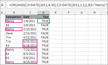
This formula nests the AND function inside the OR function to search for units sold between April 1, 2011 and January 1, 2012, or any units sold by Nancy. You can see it returns True for units sold by Nancy, and also for units sold by Tim and Ed during the dates specified in the formula.
Here’s the formula in a form you can copy and paste. If you want to play with it in a sample workbook, see the end of this article.
Use AND and OR with IF
You can also use AND and OR with the IF function.
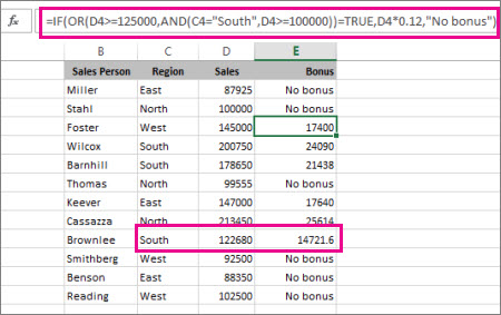
In this example, people don’t earn bonuses until they sell at least $125,000 worth of goods, unless they work in the southern region where the market is smaller. In that case, they qualify for a bonus after $100,000 in sales.
Let’s look a bit deeper. The IF function requires three pieces of data (arguments) to run properly. The first is a logical test, the second is the value you want to see if the test returns True, and the third is the value you want to see if the test returns False. In this example, the OR function and everything nested in it provides the logical test. You can read it as: Look for values greater than or equal to 125,000, unless the value in column C is «South», then look for a value greater than 100,000, and every time both conditions are true, multiply the value by 0.12, the commission amount. Otherwise, display the words «No bonus.»
Sample data
If you want to work with the examples in this article, copy the following table into cell A1 in your own spreadsheet. Be sure to select the whole table, including the heading row.
Источник
OR Function Examples IF OR Statements – Excel & Google Sheets
Download the example workbook
This tutorial demonstrates how to use the OR Function in Excel and Google Sheets to test if one or more criteria is true.
What is the OR Function?
The OR Function tests if one or more conditions are TRUE. It can evaluate up to 255 expressions.
How to Use the OR Function
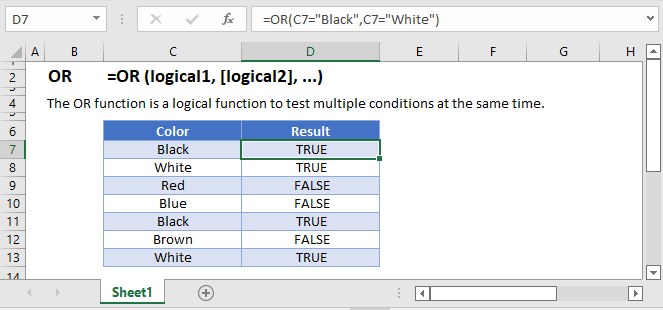
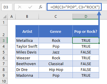
Use the Excel OR Function like this:
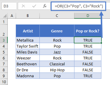
If the text in column C is equal to “Pop” or “Rock”, OR will return TRUE. Anything else will return FALSE.
Compare Text
Note that text comparisons are not case-sensitive. So the following formula would produce the same results as above:
Also, OR does not support wildcards. So this formula returns FALSE:
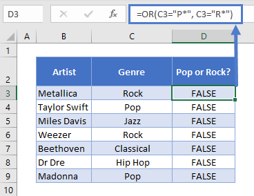
This is because OR will literally compare the text string “P*” and “R*” with the value in C3.
Compare Numbers
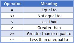
You have a range of comparison operators at your disposal when comparing numbers. These are:
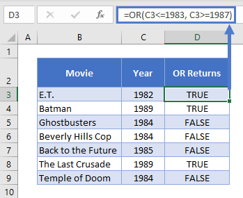
For example, if you had a list of 1980s movies and wanted to find ones from 1983 and earlier, or 1987 and later, you could use this formula:
If one of the expressions in OR is a number by itself without a comparison operator, such as =OR(1983), OR will return TRUE for that value, except if the number is zero, which evaluates to FALSE.
Using OR with Other Logical Operators
You can combine OR with any of Excel’s other logical operators, such as AND, NOT, and XOR.
Here’s how you might combine it with AND. Imagine we have a table with data on some movies. We want to find movies released after 1985 that were directed by either Steven Spielberg or Tim Burton. We could use this formula:
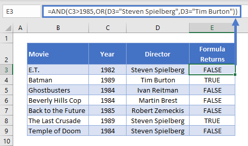
When you combine logical operators in this way, Excel works from the inside-out. So it will evaluate the OR statement here first, since that’s nested within the AND.
Using OR with IF
OR is most commonly used as part of a logical test in an IF statement.
Use it like this:
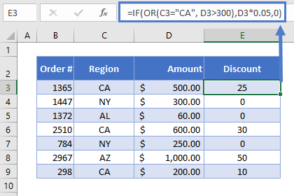
Imagine we’re running some new promotions. To help us break into the California market, we’re offering a 5% discount in that state. We’re also offering 5% off any order over $300, to encourage our customers to make bigger orders.
The IF statement evaluates our OR Function first. If returns TRUE, IF will return D3*0.05, which give us the 5% discount value. If not, it returns 0: the order didn’t meet our criteria, so we don’t apply the discount.
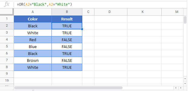
OR in Google Sheets
The OR Function works exactly the same in Google Sheets as in Excel:
OR Examples in VBA
You can also use the OR function in VBA. Type:
For the function arguments, you can either enter them directly into the function, or define variables to use instead.
Источник
OR function
Use the OR function, one of the logical functions, to determine if any conditions in a test are TRUE.
Example
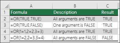
The OR function returns TRUE if any of its arguments evaluate to TRUE, and returns FALSE if all of its arguments evaluate to FALSE.
One common use for the OR function is to expand the usefulness of other functions that perform logical tests. For example, the IF function performs a logical test and then returns one value if the test evaluates to TRUE and another value if the test evaluates to FALSE. By using the OR function as the logical_test argument of the IF function, you can test many different conditions instead of just one.
The OR function syntax has the following arguments:
Required. The first condition that you want to test that can evaluate to either TRUE or FALSE.
Optional. Additional conditions that you want to test that can evaluate to either TRUE or FALSE, up to a maximum of 255 conditions.
The arguments must evaluate to logical values such as TRUE or FALSE, or in arrays or references that contain logical values.
If an array or reference argument contains text or empty cells, those values are ignored.
If the specified range contains no logical values, OR returns the #VALUE! error value.
You can use an OR array formula to see if a value occurs in an array. To enter an array formula, press CTRL+SHIFT+ENTER.
Examples
Here are some general examples of using OR by itself, and in conjunction with IF.
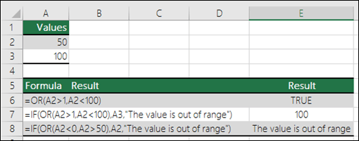
=OR(A2>1,A2 OR less than 100, otherwise it displays FALSE.
=IF(OR(A2>1,A2 OR less than 100, otherwise it displays the message «The value is out of range».
=IF(OR(A2 50),A2,»The value is out of range»)
Displays the value in cell A2 if it’s less than 0 OR greater than 50, otherwise it displays a message.
Sales Commission Calculation
Here is a fairly common scenario where we need to calculate if sales people qualify for a commission using IF and OR.
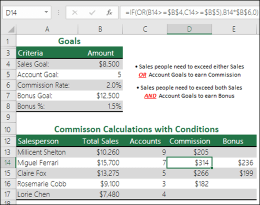
=IF(OR(B14>=$B$4,C14>=$B$5),B14*$B$6,0) — IF Total Sales are greater than or equal to (>=) the Sales Goal, OR Accounts are greater than or equal to (>=) the Account Goal, then multiply Total Sales by the Commission %, otherwise return 0.
Need more help?
You can always ask an expert in the Excel Tech Community or get support in the Answers community.
Источник
Using IF with AND, OR and NOT functions
The IF function allows you to make a logical comparison between a value and what you expect by testing for a condition and returning a result if that condition is True or False.
=IF(Something is True, then do something, otherwise do something else)
But what if you need to test multiple conditions, where let’s say all conditions need to be True or False ( AND), or only one condition needs to be True or False ( OR), or if you want to check if a condition does NOT meet your criteria? All 3 functions can be used on their own, but it’s much more common to see them paired with IF functions.
Use the IF function along with AND, OR and NOT to perform multiple evaluations if conditions are True or False.
IF(AND()) — IF(AND(logical1, [logical2], . ), value_if_true, [value_if_false]))
IF(OR()) — IF(OR(logical1, [logical2], . ), value_if_true, [value_if_false]))
IF(NOT()) — IF(NOT(logical1), value_if_true, [value_if_false]))
The condition you want to test.
The value that you want returned if the result of logical_test is TRUE.
The value that you want returned if the result of logical_test is FALSE.
Here are overviews of how to structure AND, OR and NOT functions individually. When you combine each one of them with an IF statement, they read like this:
AND – =IF(AND(Something is True, Something else is True), Value if True, Value if False)
OR – =IF(OR(Something is True, Something else is True), Value if True, Value if False)
NOT – =IF(NOT(Something is True), Value if True, Value if False)
Examples
Following are examples of some common nested IF(AND()), IF(OR()) and IF(NOT()) statements. The AND and OR functions can support up to 255 individual conditions, but it’s not good practice to use more than a few because complex, nested formulas can get very difficult to build, test and maintain. The NOT function only takes one condition.

Here are the formulas spelled out according to their logic:
=IF(AND(A2>0,B2 0,B4 50),TRUE,FALSE)
IF A6 (25) is NOT greater than 50, then return TRUE, otherwise return FALSE. In this case 25 is not greater than 50, so the formula returns TRUE.
IF A7 (“Blue”) is NOT equal to “Red”, then return TRUE, otherwise return FALSE.
Note that all of the examples have a closing parenthesis after their respective conditions are entered. The remaining True/False arguments are then left as part of the outer IF statement. You can also substitute Text or Numeric values for the TRUE/FALSE values to be returned in the examples.
Here are some examples of using AND, OR and NOT to evaluate dates.

Here are the formulas spelled out according to their logic:
IF A2 is greater than B2, return TRUE, otherwise return FALSE. 03/12/14 is greater than 01/01/14, so the formula returns TRUE.
=IF(AND(A3>B2,A3 B2,A4 B2),TRUE,FALSE)
IF A5 is not greater than B2, then return TRUE, otherwise return FALSE. In this case, A5 is greater than B2, so the formula returns FALSE.

Using AND, OR and NOT with Conditional Formatting
You can also use AND, OR and NOT to set Conditional Formatting criteria with the formula option. When you do this you can omit the IF function and use AND, OR and NOT on their own.
From the Home tab, click Conditional Formatting > New Rule. Next, select the “ Use a formula to determine which cells to format” option, enter your formula and apply the format of your choice.
 Edit Rule dialog showing the Formula method» loading=»lazy»>
Using the earlier Dates example, here is what the formulas would be.

If A2 is greater than B2, format the cell, otherwise do nothing.
=AND(A3>B2,A3 B2,A4 B2)
If A5 is NOT greater than B2, format the cell, otherwise do nothing. In this case A5 is greater than B2, so the result will return FALSE. If you were to change the formula to =NOT(B2>A5) it would return TRUE and the cell would be formatted.
Note: A common error is to enter your formula into Conditional Formatting without the equals sign (=). If you do this you’ll see that the Conditional Formatting dialog will add the equals sign and quotes to the formula — =»OR(A4>B2,A4
Need more help?

See also
You can always ask an expert in the Excel Tech Community or get support in the Answers community.
Источник
Excel for Microsoft 365 Excel for Microsoft 365 for Mac Excel for the web Excel 2021 Excel 2021 for Mac Excel 2019 Excel 2019 for Mac Excel 2016 Excel 2016 for Mac Excel 2013 Excel 2010 Excel 2007 Excel for Mac 2011 Excel Starter 2010 More…Less
Use the OR function, one of the logical functions, to determine if any conditions in a test are TRUE.
Example
The OR function returns TRUE if any of its arguments evaluate to TRUE, and returns FALSE if all of its arguments evaluate to FALSE.
One common use for the OR function is to expand the usefulness of other functions that perform logical tests. For example, the IF function performs a logical test and then returns one value if the test evaluates to TRUE and another value if the test evaluates to FALSE. By using the OR function as the logical_test argument of the IF function, you can test many different conditions instead of just one.
Syntax
OR(logical1, [logical2], …)
The OR function syntax has the following arguments:
|
Argument |
Description |
|---|---|
|
Logical1 |
Required. The first condition that you want to test that can evaluate to either TRUE or FALSE. |
|
Logical2, … |
Optional. Additional conditions that you want to test that can evaluate to either TRUE or FALSE, up to a maximum of 255 conditions. |
Remarks
-
The arguments must evaluate to logical values such as TRUE or FALSE, or in arrays or references that contain logical values.
-
If an array or reference argument contains text or empty cells, those values are ignored.
-
If the specified range contains no logical values, OR returns the #VALUE! error value.
-
You can use an OR array formula to see if a value occurs in an array. To enter an array formula, press CTRL+SHIFT+ENTER.
Examples
Here are some general examples of using OR by itself, and in conjunction with IF.
|
Formula |
Description |
|---|---|
|
=OR(A2>1,A2<100) |
Displays TRUE if A2 is greater than 1 OR less than 100, otherwise it displays FALSE. |
|
=IF(OR(A2>1,A2<100),A3,»The value is out of range») |
Displays the value in cell A3 if it is greater than 1 OR less than 100, otherwise it displays the message «The value is out of range». |
|
=IF(OR(A2<0,A2>50),A2,»The value is out of range») |
Displays the value in cell A2 if it’s less than 0 OR greater than 50, otherwise it displays a message. |
Sales Commission Calculation
Here is a fairly common scenario where we need to calculate if sales people qualify for a commission using IF and OR.
-
=IF(OR(B14>=$B$4,C14>=$B$5),B14*$B$6,0) — IF Total Sales are greater than or equal to (>=) the Sales Goal, OR Accounts are greater than or equal to (>=) the Account Goal, then multiply Total Sales by the Commission %, otherwise return 0.
Need more help?
You can always ask an expert in the Excel Tech Community or get support in the Answers community.
Related Topics
Video: Advanced IF functions
Learn how to use nested functions in a formula
IF function
AND function
NOT function
Overview of formulas in Excel
How to avoid broken formulas
Detect errors in formulas
Keyboard shortcuts in Excel
Logical functions (reference)
Excel functions (alphabetical)
Excel functions (by category)
Need more help?
Функция OR (ИЛИ) в Excel используется для сравнения двух условий.
Содержание
- Что возвращает функция
- Синтаксис
- Аргументы функции
- Дополнительная информация
- Примеры использования функции OR (ИЛИ) в Excel
- Пример 1. Используем аргументы TRUE и FALSE в функции OR (ИЛИ)
- Пример 2. Используем ссылки на ячейки, содержащих TRUE/FALSE
- Пример 3. Используем условия с функцией OR (ИЛИ)
- Пример 4. Используем числовые значения с функцией OR (ИЛИ)
- Пример 5. Используем функцию OR (ИЛИ) с другими функциями
Что возвращает функция
Возвращает логическое значение TRUE (Истина), при выполнении условий сравнения в функции и отображает FALSE (Ложь), если условия функции не совпадают.
Синтаксис
=OR(logical1, [logical2],…) — английская версия
=ИЛИ(логическое_значение1;[логическое значение2];…) — русская версия
Аргументы функции
- logical1 (логическое_значение1) — первое условие которое оценивает функция по логике TRUE или FALSE;
- [logical2] ([логическое значение2]) — (не обязательно) это второе условие которое вы можете оценить с помощью функции по логике TRUE или FALSE.
Дополнительная информация
- Функция OR (ИЛИ) может использоваться с другими формулами.
Например, в функции IF (ЕСЛИ) вы можете оценить условие и затем присвоить значение, когда данные отвечают условиям логики TRUE или FALSE. Используя функцию вместе с IF (ЕСЛИ), вы можете тестировать несколько условий оценки значений за раз.
Например, если вы хотите проверить значение в ячейке А1 по условию: “Если значение больше “0” или меньше “100” то… “ — вы можете использовать следующую формулу:
=IF(OR(A1>100,A1<0),”Верно”,”Неверно”) — английская версия
=ЕСЛИ(ИЛИ(A1>100;A1<0);»Верно»;»Неверно») — русская версия
- Аргументы функции должны быть логически вычислимы по принципу TRUE или FALSE;
- Текст и пустые ячейки игнорируются функцией;
- Если вы используете функцию с не логически вычисляемыми значениями — она выдаст ошибку;
- Вы можете тестировать максимум 255 условий в одной формуле.
Примеры использования функции OR (ИЛИ) в Excel
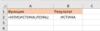
Пример 1. Используем аргументы TRUE и FALSE в функции OR (ИЛИ)

Вы можете использовать TRUE/FALSE в качестве аргументов. Если любой из них соответствует условию TRUE, функция выдаст результат TRUE. Если оба аргумента функции соответствуют условию FALSE, функция выдаст результат FALSE.
Больше лайфхаков в нашем Telegram Подписаться
Она может использовать аргументы TRUE и FALSE в кавычках.
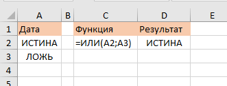
Пример 2. Используем ссылки на ячейки, содержащих TRUE/FALSE
Вы можете использовать ссылки на ячейки со значениями TRUE или FALSE. Если любое значение из ссылок соответствует условиям TRUE, функция выдаст TRUE.
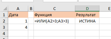
Пример 3. Используем условия с функцией OR (ИЛИ)
Вы можете проверять условия с помощью функции OR (ИЛИ). Если любое из условий соответствует TRUE, функция выдаст результат TRUE.
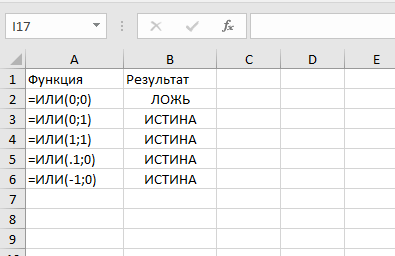
Пример 4. Используем числовые значения с функцией OR (ИЛИ)
Число “0” считается FALSE в Excel по умолчанию. Любое число, выше “0”, считается TRUE (оно может быть положительным, отрицательным или десятичным числом).
Пример 5. Используем функцию OR (ИЛИ) с другими функциями
Вы можете использовать функцию OR (ИЛИ) с другими функциями для того, чтобы оценить несколько условий.
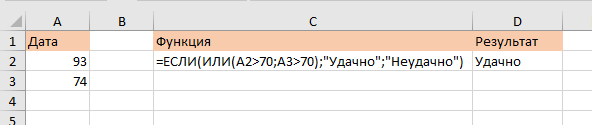
На примере ниже показано, как использовать функцию вместе с IF (ЕСЛИ):
На примере выше, мы дополнительно используем функцию IF (ЕСЛИ) для того, чтобы проверить несколько условий. Формула проверяет значение ячеек А2 и A3. Если в одной из них значение более чем “70”, то формула выдаст “TRUE”.
На чтение 2 мин Просмотров 337 Опубликовано 10.12.2021
Эта функция поможет вам в том случае, когда необходимо проверить несколько логических условий.
Содержание
- Что возвращает функция ИЛИ (OR)?
- Синтаксис
- Важная информация
- Варианты использования ИЛИ
- Аргументы ИСТИНА и ЛОЖЬ прямо в формуле функции ИЛИ
- Аргументы ИСТИНА и ЛОЖЬ в ячейках на которые ссылаются аргументы функции ИЛИ
- Условия в аргументах функции
- Использование функции ИЛИ с числами
- Комбинируем функцию ИЛИ с другими функциями Excel
Что возвращает функция ИЛИ (OR)?
Если любое из условий, в аргументах функции, имеет значение ИСТИНА, то возвращает ИСТИНА, если нет, то ЛОЖЬ.
Синтаксис
=ИЛИ(любой_аргумент_имеющий_логическое_значение1; [любой_аргумент_имеющий_логическое_значение2];...)Аргументами могут быть и вычисления — например, 1+1=2 — ИСТИНА.
Важная информация
- Комбинация функций ЕСЛИ и ИЛИ позволяет проверить несколько логических утверждений за один вызов этих функций. Например, необходимо узнать, больше ли значение ячейки A1 чем 0 или меньше 100, в таком случае: =ЕСЛИ(ИЛИ(A1>100;A1<0); «Да»; «Нет»);
- Обычный текст или пустые значения ячеек не сработают в аргументах функции;
- Если аргументами функции не являются логически значения то функция выдаст ошибку #ЗНАЧ!;
- Максимально, в аргументах, можно указать 255 значений.
Варианты использования ИЛИ
Давайте рассмотрим несколько вариантов использования функции
Аргументы ИСТИНА и ЛОЖЬ прямо в формуле функции ИЛИ
Итак, как я уже говорил ранее, функция сравнивает каждое логическое значение и если находит ИСТИНУ, то возвращает ИСТИНА, если нет, то ЛОЖЬ. Если в первом аргументе функции вы использовали ИСТИНА, то вернется, соответственно, ИСТИНА.
Аргументы ИСТИНА и ЛОЖЬ в ячейках на которые ссылаются аргументы функции ИЛИ
Тоже самое что и в примере выше, только мы используем ссылки на ячейки с логическими значениями.
Условия в аргументах функции
Вы можете проверять какие-либо утверждения в аргументах функции.

Использование функции ИЛИ с числами
Если вы читаете статьи нашего сайта, вы знаете что все числа в Excel обладают логическими значениями. 0 — Ложь, а все остальные числа — ИСТИНА. Таким образом мы можем указывать числа в аргументах функции.
Комбинируем функцию ИЛИ с другими функциями Excel
И конечно же, можно комбинировать нашу функцию с другими функциями Excel. Наверное, это самый распространенный вариант использования.
Пример на картинке ниже:
Итак, наша функция проверяет больше ли значение ячейки A2 чем число 70, или значение ячейки A3 чем 70. Если любое из этих утверждений будет верно, результатом выполнения функции будет «Удачно», если же нет — «Неудачно».

| Раздел функций | Логические |
| Название на английском | OR |
| Волатильность | Не волатильная |
| Похожие функции | И, НЕ, ЕСЛИ |
Что делает функция ИЛИ?
Эта функция проверяет два или более условий, чтобы проверить, верно ли хотя бы одно из них. Выражаясь математическим языком, производит операцию дизъюнкции.
Критерии сравнения, которые можно использовать: ‘=’ (равно), ‘>’ (больше), ‘<‘ (меньше), ‘<>’ (не равно), ‘>=’ (больше или равно), ‘<=’ (меньше или равно). Сравнивать можно и логические, и цифровые, и текстовые значения.
Обычно функция ИЛИ используется в паре другими логическими, наиболее часто с функцией ЕСЛИ.
Синтаксис
=ИЛИ(Выражение1;Выражение2;…)
Значок ИЛИ в Excel (“∪”) можно получить с помощью функции ЮНИСИМВ.

=ЮНИСИМВ(8746)
Это не оператор, а обычный текстовый символ. Он может быть использован исключительно для текстовой записи математических выражений.
Форматирование
Функция корректно обработает:
- Числа и вычисления, возвращающие их
- Логические выражения (ИСТИНА, ЛОЖЬ) и вычисления, возвращающие их
- Ячейки, содержащие их
- Диапазоны ячеек, если хотя бы одна ячейка содержит числа, ИСТИНА или ЛОЖЬ
- Массивы значений или вычислений
Если на вход подается диапазон, в значениях которого присутствуют текстовые значения, они не учитываются функцией, как и пустые ячейки.
Функция выдаст ошибку, если:
- на вход получены только текстовые или пустые ячейки (одна или несколько)
- среди значений есть ошибки (#ЗНАЧ!, #Н/Д, #ИМЯ?, #ПУСТО!, #ДЕЛ/0!, #ССЫЛКА!, #ЧИСЛО!)
Примеры применения
Пример 1
Как правило, если слово состоит из только гласных или только согласных букв – это аббревиатура
Воспользуемся комбинацией – функция ИЛИ + функция ЕЧИСЛО + функция ПОИСК, чтобы определить на основе этого признака, что слово является аббревиатурой
Это поможет нам далее исправить регистр слова функцией ПРОПИСН, если оно изначально написано в нижнем.
Составим формулы массива для поиска гласных и согласных букв.

Теперь составим общую формулу проверки.
Для того, чтобы соблюдалось условие аббревиатуры, условия наличия гласных и согласных должны противоречить друг другу
Т.е. есть гласные и нет согласных, или, наоборот, есть согласные, но нет гласных.
Самым коротким способом записать это можно функцией НЕ.

Пример 2
Студенты получают оценки в виде букв A-F, каждая из букв может быть с плюсом. “F” и “F+” – неудовлетворительные оценки. Задача с помощью одной формулы узнать, нужна ли студенту пересдача.

Почему фигурные скобки в формуле присутствуют дважды?
Используется массив внутри формулы массива – таблица оценок студента сравнивается с массивом строковых констант “F” и “F+”.
Столбец оценок – вертикальный, а массив строковых констант – горизонтальный. При сравнении этих двух массивов (в скобках) , возвращается массив булевых значений размерностью 5 на 2.
Функция ИЛИ возвращает ИСТИНА, если в этом массиве есть хотя бы одна неудовлетворительная оценка.
Файл с примерами применения функции ИЛИ
Ниже интерактивный файл с примерами. Попробуйте поменять значения в ячейках. С помощью двойного клика по ячейке с формулой можно ее просмотреть, скопировать или отредактировать. Можно скачать файл для использования на собственном компьютере.
Другие логические функции
ЕСЛИ, И, НЕ