Excel rows to repeat

Repeat specific rows or columns on every printed page

If a worksheet spans more than one printed page, you can label data by adding row and column headings that will appear on each print page. These labels are also known as print titles.

Follow these steps to add Print Titles to a worksheet:

On the worksheet that you want to print, in the Page Layout tab, click Print Titles , in the Page Setup group.

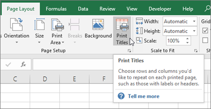
Note: The Print Titles command will appear dimmed if you are in cell editing mode, if a chart is selected on the same worksheet, or if you don’t have a printer installed. For more information about installing a printer, see finding and installing printer drivers for Windows Vista. Please note that Microsoft has discontinued support for Windows XP; check your printer manufacturer’s Web site for continued driver support.

On the Sheet tab, under Print titles, do one—or both—of the following:

In the Rows to repeat at top box, enter the reference of the rows that contain the column labels.

In the Columns to repeat at left box, enter the reference of the columns that contain the row labels.

For example, if you want to print column labels at the top of every printed page, you could type $1:$1 in the Rows to repeat at top box.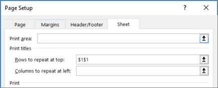

Tip: You can also click the Collapse Popup Window buttons at the right end of the Rows to repeat at top and Columns to repeat at left boxes, and then select the title rows or columns that you want to repeat in the worksheet. After you finish selecting the title rows or columns, click the Collapse Dialog button again to return to the dialog box.

Note: If you have more than one worksheet selected, the Rows to repeat at top and Columns to repeat at left boxes are not available in the Page Setup dialog box. To cancel a selection of multiple worksheets, click any unselected worksheet. If no unselected sheet is visible, right-click the tab of a selected sheet, and then click Ungroup Sheets on the shortcut menu.

Источник

How to Insert Multiple Rows in Excel

In the last few decades, Microsoft has grown by leaps and bounds and so are its fabulous products. Microsoft Excel is one such product that has grown immensely. It has wonderful features and options to make your tasks easier. But one feature that it lacks is the ability to insert multiple rows. The default insert option that Excel has allows you to insert only one row at a time.

This can be very annoying in cases where you have to insert multiple rows in your spreadsheet. And this is what I am going to write today. In this post, I will present a few ways which allow you to insert multiple rows.

Table of Contents

Method 1 – By making use of the repeat functionality of excel:

This is the simplest way to insert multiple rows in your excel spreadsheet. In this method, we will first add one row manually to the excel sheet then repeat that action multiple times. Follow the below steps to use this method:

• Open your spreadsheet, and first of all insert one row to your excel sheet manually.
• Then simply repeatedly press the “F4” key on your keyboard, till the required number of rows are inserted.
• This will repeat your last action and the rows will be added.

Method 2 – By using the insert functionality:

In this method, we will use a hidden feature that excel offers to insert multiple rows to your sheet. Follow the below steps to use this method:

• Open your spreadsheet and select the number of rows that you want to insert to your sheet. It doesn’t matter if the rows are empty but they must include the place where you want to perform the insert.

• Now simply right-click anywhere in the previously selected range and select the ‘Insert’ option.
• Now excel will ask you whether to shift the cells down or shift them to right. Select the option ‘Shift Cells Down’ and multiple cells will be inserted in the location.

Method 3 – By using the insert copied cells functionality:

In this method, we are going to take the advantage of the “Insert Copied Cells” functionality that excel has. Follow the below steps to use this method:

• First of all select multiple rows in your spreadsheet, by multiple I mean they should be equal to the number of rows that you want to insert.
• Next, copy these rows and scroll to the place where you want to insert multiple rows.

• Right-click and select the option ‘Insert Copied Cells’ and this will insert multiple rows at that place.

Method 4 – Programmatically inserting multiple rows in excel:

Although this method is a bit complex than the first three, still this can be used if you are more inclined towards the coding side. Follow the below steps to use this method:

• Navigate to the ‘View’ tab on the top ribbon, click on the ‘Macros’ button.
• Now type the name for the macro say “Insert_Lines” (without quotes) and hit the create button.
• Next, a VBA editor will be opened, simply paste the below macro code after the first line.

• Now comes the important thing, in the above macro the range is (“A20:A69”). The first parameter i.e. A20 tells the position from where you wish to insert the rows and the second parameter .i.e. A69 is the number of rows to be inserted added with the start position and subtracted by 1 (for instance: If you want to insert 50 rows starting from A20 then the second parameter of the range should be (50+20-1), so the range will be (“A20:A69”))
• After adding the code you can press the “F5” key and the code will insert the required rows.
• This macro is referenced from the Microsoft article: http://support.microsoft.com/kb/291305

So, these were the few methods to insert multiple rows in excel. If you know some other ways then feel free to comment below.

Subscribe and be a part of our 15,000+ member family!

Now subscribe to Excel Trick and get a free copy of our ebook «200+ Excel Shortcuts» (printable format) to catapult your productivity.

Источник

Repeating Rows in Excel

When your Excel spreadsheet spans several pages, the data is easier to follow when you print the column titles at the top of every page. Instead of manually repeating the title row, you can command Excel to automatically repeat the row on every page using the Print Titles feature. Excel also includes features that make it easier to repeat rows when you’re entering duplicate data into the spreadsheet.

Title Rows

Click the «Page Layout» tab, and select «Print Titles» from the Page Setup section of the ribbon.

Click inside the box next to «Rows to Repeat at Top» in the Page Setup dialog box.

Click in the worksheet on the row you want to repeat. The cell values appear automatically in the dialog box.

Click «OK» to save the change and close the dialog box. The row you selected appears at the top of every page when you print the worksheet.

Duplicate Rows

Select the row or rows you want to repeat.

Move your pointer over the small square fill handle in the bottom left corner of the selection area so that the pointer turns into a black «+» sign.

Drag the fill handle down over the rows into which you copy the original data, and then release the mouse button. Excel automatically fills the rows with the repeated data. If you already have data in the other rows that you don’t want to copy over, use the next method instead.

Select the row or rows you want to repeat. Right-click the selection and click «Copy.»

Select the rows into which you want to copy the original row or rows. Right-click the selection, and then click «Insert Copied Cells.» Excel inserts the repeated data into the new rows, moving the existing rows down.

Источник

How to delete empty rows in Excel quickly

When importing and copying tables in Excel, empty strings and cells can be formed. They always district and interfere with the work.

Some formulas may not work correctly. It is impossible to use a number of tools for an incompletely filled range. We will learn how to quickly delete empty cells at the end or middle of a table. We will use simple tools available to the user of any level.

How to remove empty rows in the Excel table?

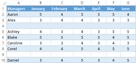
To show you how to delete extra lines, to illustrate the order of actions, take a table with conditional data:

Example 1: Sorting data in a table. Select the entire table. Open the «DATA» tab — «Sort and Filter» tool — press the «Sort» button. Another way is to right-click on the selected range and do the sorting «A to Z».

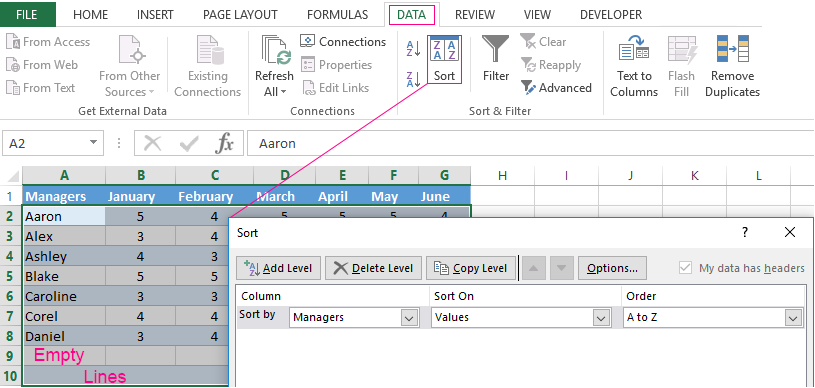
Empty rows after sorting in ascending order are at the bottom of the range.

If the order of the values is important, then before the sorting, you need to insert an empty column, make a through numbering. After sorting and deleting blank lines, sort the data by the inserted column with the numbering again.

Example 2: Filter. The range must be formatted as a table with headers. We select the «cap». On the «DATA» tab, we click the «Filter» button («Sort and Filter»). A down arrow appears to the right of each column name. Push — opens the filtering window. Remove the selection in front of the name «Empty».

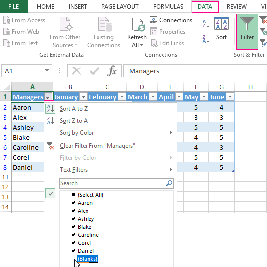
You can delete empty cells in the Excel line the same way. Select the required column and filter its data.

Example 3: Selecting a group of cells. Select the entire table. In the main menu on the «Edit» tab we click the button «Find and Select». Select the «Go To Special» tool. In the window that opens, select the «Blanks».

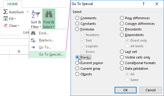
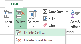
The program marks empty cells. On the main page we find the «HOME»-«Delete»-«Delete Cells».

The result is a filled range of «no voids».

Attention! After the removal, some of the cells jump upwards — the data can be messed up. Therefore, for the overlapping ranges, the instrument is not suitable.

Helpful advice! The shortcut to delete the selected row in Excel is CTRL + «-«. And for its selection, you can press the hotkey combination SHIFT + SPACEBAR.

How to remove repeated rows in Excel?

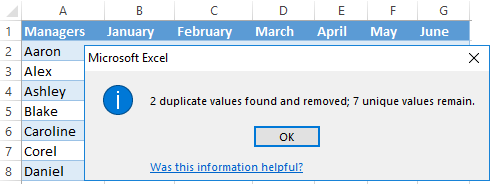
To remove the same rows in Excel, select the entire table. Go to the tab «DATA»-«Data Tool»-«Delete Duplicates».

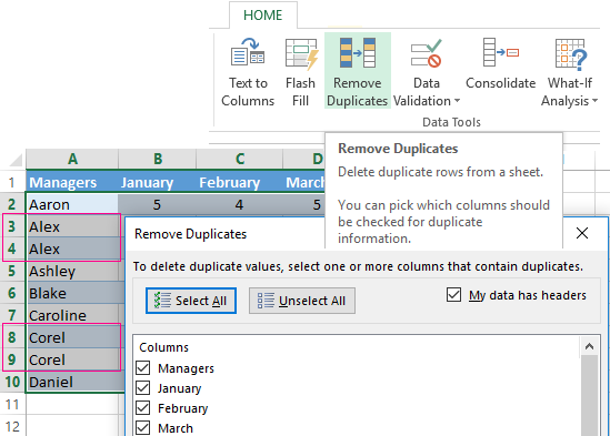
In the window that opens, select those columns that contain duplicate values. Since you need to delete duplicate rows, all columns should be highlighted. After clicking OK Excel creates a mini-report of the form:

How to remove each second line in Excel?

You can use the macro to break the table. For example, this:

Sub Delete_Every_Other_Row()
‘ Dimension variables.
Y = False ‘ Change this to True if you want to
‘ delete rows 1, 3, 5, and so on.
I = 1
Set xRng = Selection
‘ Loop once for every row in the selection.
For xCounter = 1 To xRng.Rows.Count
‘ If Y is True, then.
If Y = True Then
‘ . delete an entire row of cells.
xRng.Cells(I).EntireRow.Delete
‘ Otherwise.
Else
‘ . increment I by one so we can cycle through range.
I = I + 1
End If
‘ If Y is True, make it False; if Y is False, make it True.
Y = Not Y
Next xCounter
End Sub

And you can do it by hand. We offer a simple way, accessible to each user.

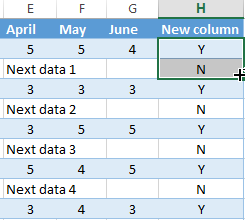
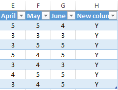
1. At the end of the table, make an auxiliary column. Fill with alternate data. For example, «N Y N Y», etc. We enter values in the first four cells. Then select them. «We catch» for the black cross in the lower right corner and copy the letters to the end of the range.
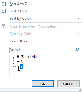
2. Install the «Filter». Filter the last column by the value of «Y».
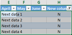
3. Select all that is left after filtering and delete.
4. We remove the filter — only cells with «N» will remain.

The auxiliary column can be eliminated and operated with a «decimated table».

When the user had hidden some information in the rows he was not distracted from his work. I thought that later the data would be needed. It is not needed — hidden rows can be deleted: they affect the formulas, interfere.

In the training table are hidden rows 5, 6, 7:

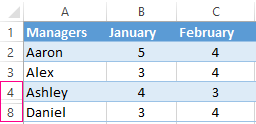
We will remove them.

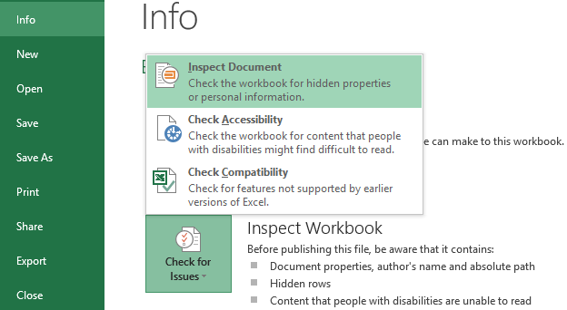
1. Go to «FILE»-«Info»-«Check for Issues» the tool «Inspect Document».
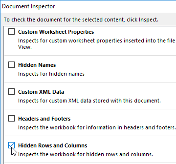
2. In the opened window, put a tick in front of the «Hidden Rows and Columns». Click «Inspect».
3. After a few seconds, the program displays the result of the test.
4. Click «Remove All». A corresponding notification will appear on the screen.

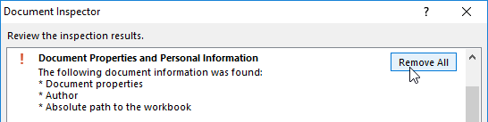
As a result of the work done, the hidden cells are deleted, the numbering is restored.

Thus, remove the empty, repeating or hidden cells of the table using the built-in functionality of the Excel program.

Источник