
Excel 2021 Excel 2019 Excel 2016 Excel 2013 Office for business Excel 2010 More…Less
Summary
When you use the Microsoft Excel products listed at the bottom of this article, you can use a worksheet formula to covert data that spans multiple rows and columns to a database format (columnar).
More Information
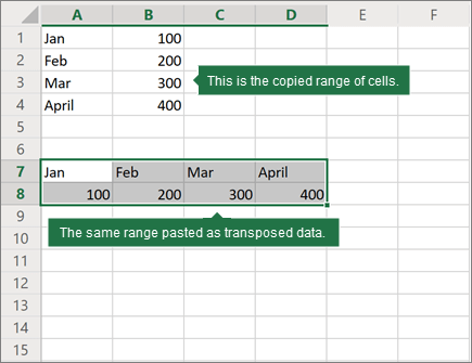
The following example converts every four rows of data in a column to four columns of data in a single row (similar to a database field and record layout). This is a similar scenario as that which you experience when you open a worksheet or text file that contains data in a mailing label format.
Example
-
In a new worksheet, type the following data:
A1: Smith, John
A2: 111 Pine St.
A3: San Diego, CA
A4: (555) 128-549
A5: Jones, Sue
A6: 222 Oak Ln.
A7: New York, NY
A8: (555) 238-1845
A9: Anderson, Tom
A10: 333 Cherry Ave.
A11: Chicago, IL
A12: (555) 581-4914 -
Type the following formula in cell C1:
=OFFSET($A$1,(ROW()-1)*4+INT((COLUMN()-3)),MOD(COLUMN()-3,1))
-
Fill this formula across to column F, and then down to row 3.
-
Adjust the column sizes as necessary. Note that the data is now displayed in cells C1 through F3 as follows:
Smith, John
111 Pine St.
San Diego, CA
(555) 128-549
Jones, Sue
222 Oak Ln.
New York, NY
(555) 238-1845
Anderson, Tom
333 Cherry Ave.
Chicago, IL
(555) 581-4914
The formula can be interpreted as
OFFSET($A$1,(ROW()-f_row)*rows_in_set+INT((COLUMN()-f_col)/col_in_set), MOD(COLUMN()-f_col,col_in_set))
where:
-
f_row = row number of this offset formula
-
f_col = column number of this offset formula
-
rows_in_set = number of rows that make one record of data
-
col_in_set = number of columns of data
Need more help?
Want more options?
Explore subscription benefits, browse training courses, learn how to secure your device, and more.
Communities help you ask and answer questions, give feedback, and hear from experts with rich knowledge.
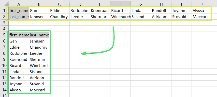
Do you have some values arranged as rows in your workbook, and do you want to convert text in rows to columns in Excel like this?
In Excel, you can do this manually or automatically in multiple ways depending on your purpose. Read on to get all the details and choose the best solution for yourself.
How to convert rows into columns or columns to rows in Excel – the basic solution
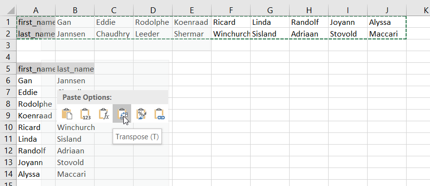
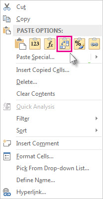
The easiest way to convert rows to columns in Excel is via the Paste Transpose option. Here is how it looks:
- Select and copy the needed range
- Right-click on a cell where you want to convert rows to columns
- Select the Paste Transpose option to rotate rows to columns
As an alternative, you can use the Paste Special option and mark Transpose using its menu.

It works the same if you need to convert columns to rows in Excel.

This is the best way for a one-time conversion of small to medium numbers of rows both in the Excel desktop and online.
Can I convert multiple rows to columns in Excel from another workbook?
The method above will work well if you want to convert rows to columns in Excel between different workbooks using Excel desktop. You need to have both spreadsheets open and do the copying and pasting as described.
However, in Excel Online, this won’t work for different workbooks. The Paste Transpose option is not available.
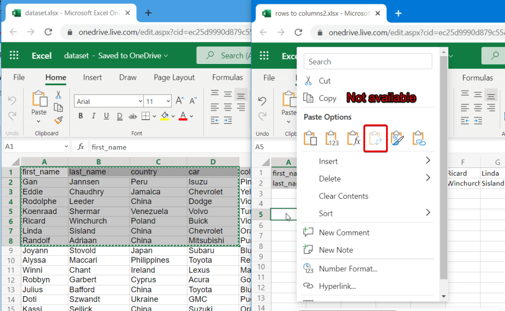
Therefore, in this case, it’s better to use the TRANSPOSE function.
How to switch rows and columns in Excel in more efficient ways
To switch rows and columns in Excel automatically or dynamically, you can use one of these options:
- Excel TRANSPOSE function
- VBA macro
- Power Query
Let’s check out each of them in the example of a data range that we imported to Excel from a Google Sheets file using Coupler.io.

Coupler.io is an integration solution that synchronizes data between source and destination apps on a regular schedule. For example, you can set up an automatic data export from Google Sheets every day to your Excel workbook.
Check out all the available Excel integrations.

How to change row to column in Excel with TRANSPOSE
TRANSPOSE is the Excel function that allows you to switch rows and columns in Excel. Here is its syntax:
=TRANSPOSE(array)array– an array of columns or rows to transpose
One of the main benefits of TRANSPOSE is that it links the converted columns/rows with the source rows/columns. So, if the values in the rows change, the same changes will be made in the converted columns.
TRANSPOSE formula to convert multiple rows to columns in Excel desktop
TRANSPOSE is an array formula, which means that you’ll need to select a number of cells in the columns that correspond to the number of cells in the rows to be converted and press Ctrl+Shift+Enter.
=TRANSPOSE(A1:J2)
Fortunately, you don’t have to go through this procedure in Excel Online.
TRANSPOSE formula to rotate row to column in Excel Online
You can simply insert your TRANSPOSE formula in a cell and hit enter. The rows will be rotated to columns right away without any additional button combinations.
Excel TRANSPOSE multiple rows in a group to columns between different workbooks
We promised to demonstrate how you can use TRANSPOSE to rotate rows to columns between different workbooks. In Excel Online, you need to do the following:
- Copy a range of columns to rotate from one spreadsheet and paste it as a link to another spreadsheet.

- We need this URL path to use in the TRANSPOSE formula, so copy it.

- The URL path above is for a cell, not for an array. So, you’ll need to slightly update it to an array to use in your TRANSPOSE formula. Here is what it should look like:
=TRANSPOSE('https://d.docs.live.net/ec25d9990d879c55/Docs/Convert rows to columns/[dataset.xlsx]dataset'!A1:D12)

You can follow the same logic for rotating rows to columns between workbooks in Excel desktop.
Are there other formulas to convert columns to rows in Excel?
TRANSPOSE is not the only function you can use to change rows to columns in Excel. A combination of INDIRECT and ADDRESS functions can be considered as an alternative, but the flow to convert rows to columns in Excel using this formula is much trickier. Let’s check it out in the following example.
How to convert text in columns to rows in Excel using INDIRECT+ADDRESS
If you have a set of columns with the first cell A1, the following formula will allow you to convert columns to rows in Excel.
=INDIRECT(ADDRESS(COLUMN(A1),ROW(A1)))

But where are the rows, you may ask! Well, first you need to drag this formula down if you are converting multiple columns to rows. Then drag it to the right.

NOTE: This Excel formula only to convert data in columns to rows starting with A1 cell. If your columns start from another cell, check out the next section.
How to convert Excel data in columns to rows using INDIRECT+ADDRESS from other cells
To convert columns to rows in Excel with INDIRECT+ADDRESS formulas from not A1 cell only, use the following formula:
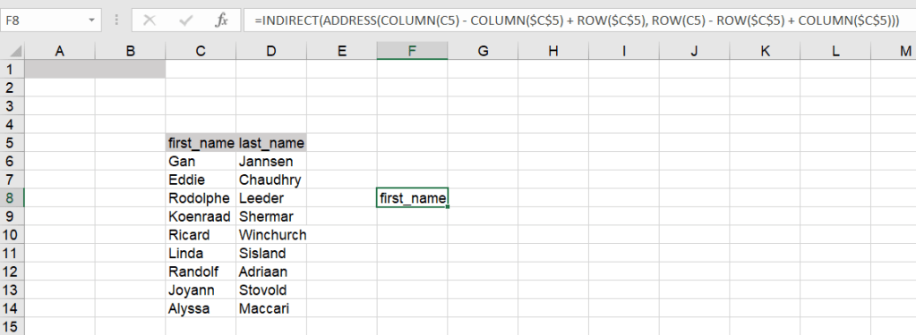
=INDIRECT(ADDRESS(COLUMN(first_cell) - COLUMN($first_cell) + ROW($first_cell), ROW(first_cell) - ROW($first_cell) + COLUMN($first_cell)))
- first_cell – enter the first cell of your columns
Here is an example of how to convert Excel data in columns to rows:
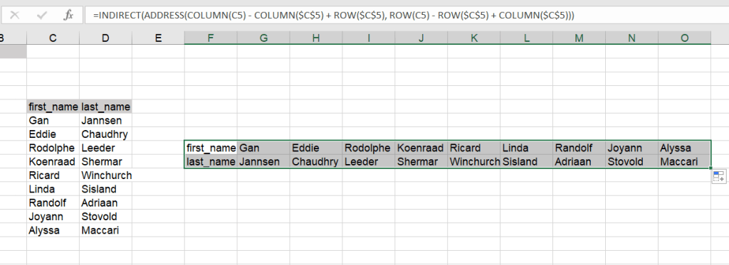
=INDIRECT(ADDRESS(COLUMN(C5) - COLUMN($C$5) + ROW($C$5), ROW(C5) - ROW($C$5) + COLUMN($C$5)))
Again, you’ll need to drag the formula down and to the right to populate the rest of the cells.
How to automatically convert rows to columns in Excel VBA
VBA is a superb option if you want to customize some function or functionality. However, this option is only code-based. Below we provide a script that allows you to change rows to columns in Excel automatically.
- Go to the Visual Basic Editor (VBE). Click Alt+F11 or you can go to the Developer tab => Visual Basic.

- In VBE, go to Insert => Module.
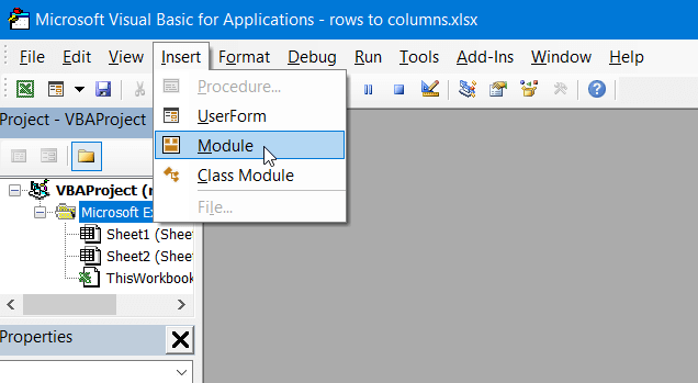
- Copy and paste the script into the window. You’ll find the script in the next section.

- Now you can close the VBE. Go to Developer => Macros and you’ll see your RowsToColumns macro. Click Run.

- You’ll be asked to select the array to rotate and the cell to insert the rotated columns.

- There you go!

VBA macro script to convert multiple rows to columns in Excel
Sub TransposeColumnsRows()
    Dim SourceRange As Range
    Dim DestRange As Range

    Set SourceRange = Application.InputBox(Prompt:="Please select the range to transpose", Title:="Transpose Rows to Columns", Type:=8)
    Set DestRange = Application.InputBox(Prompt:="Select the upper left cell of the destination range", Title:="Transpose Rows to Columns", Type:=8)

    SourceRange.Copy
    DestRange.Select
    Selection.PasteSpecial Paste:=xlPasteAll, Operation:=xlNone, SkipBlanks:=False, Transpose:=True
    Application.CutCopyMode = False

End Sub

Sub RowsToColumns()
    Dim SourceRange As Range
    Dim DestRange As Range

    Set SourceRange = Application.InputBox(Prompt:="Select the array to rotate", Title:="Convert Rows to Columns", Type:=8)
    Set DestRange = Application.InputBox(Prompt:="Select the cell to insert the rotated columns", Title:="Convert Rows to Columns", Type:=8)

    SourceRange.Copy
    DestRange.Select
    Selection.PasteSpecial Paste:=xlPasteAll, Operation:=xlNone, SkipBlanks:=False, Transpose:=True
    Application.CutCopyMode = False

End Sub
Read more in our Excel Macros Tutorial.
Convert rows to column in Excel using Power Query
Power Query is another powerful tool available for Excel users. We wrote a separate Power Query Tutorial, so feel free to check it out.
Meanwhile, you can use Power Query to transpose rows to columns. To do this, go to the Data tab, and create a query from table.

- Then select a range of cells to convert rows to columns in Excel. Click OK to open the Power Query Editor.

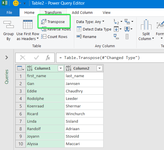
- In the Power Query Editor, go to the Transform tab and click Transpose. The rows will be rotated to columns.
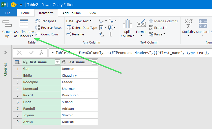
- If you want to keep the headers for your columns, click the Use First Row as Headers button.
- That’s it. You can Close & Load your dataset – the rows will be converted to columns.

Error message when trying to convert rows to columns in Excel
To wrap up with converting Excel data in columns to rows, let’s review the typical error messages you can face during the flow.
Overlap error

The overlap error occurs when you’re trying to paste the transposed range into the area of the copied range. Please avoid doing this.
Wrong data type error

You may see this #VALUE! error when you implement the TRANSPOSE formula in Excel desktop without pressing Ctrl+Shift+Enter.
Other errors may be caused by typos or other misprints in the formulas you use to convert groups of data from rows to columns in Excel. Always double-check the syntax before pressing Enter or Ctrl+Shift+Enter 🙂 . Good luck with your data!
-

A content manager at Coupler.io whose key responsibility is to ensure that the readers love our content on the blog. With 5 years of experience as a wordsmith in SaaS, I know how to make texts resonate with readers’ queries✍🏼

Back to Blog
Focus on your business
goals while we take care of your data!
Try Coupler.io
Summary
To flip a table in Excel from rows to columns (i.e. to change orientation from vertical to horizontal) you can use the TRANSPOSE function.
In the example shown the formula in E5:K6 is:
{=TRANSPOSE(B5:C11)}
Note: this is a multi-cell array formula and must be entered with Control + Shift + Enter.
Generic formula
Explanation
The TRANSPOSE function is fully automatic and can transpose cells vertical to horizontal, and vice versa. The only requirement is that there be a one to one relationship between source and target cells.
In the example shown, we are transposing a table that is 2 columns by 7 rows (14 cells), to a table that is 7 columns by 2 rows (14 cells).
Note that this function creates a dynamic link between the source and target. Any change in to data in the source table will be reflected in the target table.
One-off conversion with Paste Special
If you simply need to do a one-time conversion, and don’t need dynamic links, you can use Paste Special. Select the source data, copy, then use Paste Special > Transpose.

Author![]()
Dave Bruns
Hi — I’m Dave Bruns, and I run Exceljet with my wife, Lisa. Our goal is to help you work faster in Excel. We create short videos, and clear examples of formulas, functions, pivot tables, conditional formatting, and charts.
There are hundreds and hundreds of Excel sites out there. I’ve been to many and most are an exercise in frustration. Found yours today and wanted to let you know that it might be the simplest and easiest site that will get me where I want to go.
Get Training
Quick, clean, and to the point training
Learn Excel with high quality video training. Our videos are quick, clean, and to the point, so you can learn Excel in less time, and easily review key topics when needed. Each video comes with its own practice worksheet.
View Paid Training & Bundles
Help us improve Exceljet
Quick and simple ways to convert row to column in Excel. read on to know how.
It might happen that you are working on a sheet where you have some values arranged as rows and you want to convert the text in rows to columns in Excel as shown in the picture below.

Excel allows you to do this manually or automatically in several ways depending on your purpose.
Let us learn how to convert rows to columns in Excel.
How to Convert Row To Column in Excel – The Basic Solution
The easiest way to do it is via the Paste Transpose option. Here is how:
- Select and copy the needed range
- Right-click on a cell where you want to convert rows to columns
- Select the Paste Transpose option to rotate rows to columns

You can also use the Paste Special option and mark Transpose using its menu.

How to change row to column in Excel with TRANSPOSE
TRANSPOSE is the Excel function that allows you to switch rows and columns in Excel. Here is its syntax:
=TRANSPOSE(array)
- array – an array of columns or rows to transpose
The benefit of TRANSPOSE is that it links the converted columns/rows with the source rows/columns. So, if the values in the rows change, the same changes will be made in the converted columns.
TRANSPOSE formula to convert multiple rows to columns in Excel desktop
TRANSPOSE is an array formula, which means that you’ll need to select a number of cells in the columns that correspond to the number of cells in the rows to be converted and press Ctrl+Shift+Enter.
=TRANSPOSE(A1:J2)

TRANSPOSE formula to rotate row to column in Excel Online
Insert your TRANSPOSE formula in a cell and hit enter. The rows will be rotated to columns.

Excel TRANSPOSE multiple rows in a group to columns between different workbooks
To use TRANSPOSE to rotate rows to columns between different workbooks, do the following:
- Copy a range of columns to rotate from one spreadsheet and paste it as a link to another spreadsheet.

- Copy the URL path.

- The URL path above is for a cell, not for an array. So, you’ll need to slightly update it to an array to use in your TRANSPOSE formula. Here is what it should look like:
=TRANSPOSE(‘https://d.docs.live.net/ec25d9990d879c55/Docs/Convert rows to columns/[dataset.xlsx]dataset’!A1:D12)

Follow the same logic for rotating rows to columns between workbooks on an Excel desktop.
Содержание
- TRANSPOSE function
- Step 1: Select blank cells
- Step 2: Type =TRANSPOSE(
- Step 3: Type the range of the original cells.
- Step 4: Finally, press CTRL+SHIFT+ENTER
- Technical details
- Syntax
- Transpose (rotate) data from rows to columns or vice versa
- Tips for transposing your data
- Need more help?
- How You Can Convert Rows to Columns or Columns to Rows in Excel Workbooks
- How to convert rows into columns or columns to rows in Excel – the basic solution
- Can I convert multiple rows to columns in Excel from another workbook?
- How to switch rows and columns in Excel in more efficient ways
- How to change row to column in Excel with TRANSPOSE
- TRANSPOSE formula to convert multiple rows to columns in Excel desktop
- TRANSPOSE formula to rotate row to column in Excel Online
- Excel TRANSPOSE multiple rows in a group to columns between different workbooks
- Are there other formulas to convert columns to rows in Excel?
- How to convert text in columns to rows in Excel using INDIRECT+ADDRESS
- How to convert Excel data in columns to rows using INDIRECT+ADDRESS from other cells
- How to automatically convert rows to columns in Excel VBA
- VBA macro script to convert multiple rows to columns in Excel
- Convert rows to column in Excel using Power Query
- Error message when trying to convert rows to columns in Excel
- Overlap error
- Wrong data type error
TRANSPOSE function
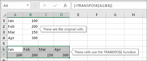
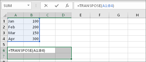
Sometimes you need to switch or rotate cells. You can do this by copying, pasting, and using the Transpose option. But doing that creates duplicated data. If you don’t want that, you can type a formula instead using the TRANSPOSE function. For example, in the following picture the formula =TRANSPOSE(A1:B4) takes the cells A1 through B4 and arranges them horizontally.
Note: If you have a current version of Microsoft 365 , then you can input the formula in the top-left-cell of the output range, then press ENTER to confirm the formula as a dynamic array formula. Otherwise, the formula must be entered as a legacy array formula by first selecting the output range, input the formula in the top-left-cell of the output range, then press Ctrl+Shift+Enter to confirm it. Excel inserts curly brackets at the beginning and end of the formula for you. For more information on array formulas, see Guidelines and examples of array formulas.
Step 1: Select blank cells
First select some blank cells. But make sure to select the same number of cells as the original set of cells, but in the other direction. For example, there are 8 cells here that are arranged vertically:

So, we need to select eight horizontal cells, like this:

This is where the new, transposed cells will end up.
Step 2: Type =TRANSPOSE(
With those blank cells still selected, type: =TRANSPOSE(
Excel will look similar to this:
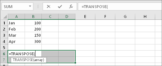
Notice that the eight cells are still selected even though we have started typing a formula.
Step 3: Type the range of the original cells.
Now type the range of the cells you want to transpose. In this example, we want to transpose cells from A1 to B4. So the formula for this example would be: =TRANSPOSE(A1:B4) — but don’t press ENTER yet! Just stop typing, and go to the next step.
Excel will look similar to this:
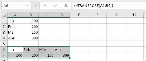
Step 4: Finally, press CTRL+SHIFT+ENTER
Now press CTRL+SHIFT+ENTER. Why? Because the TRANSPOSE function is only used in array formulas, and that’s how you finish an array formula. An array formula, in short, is a formula that gets applied to more than one cell. Because you selected more than one cell in step 1 (you did, didn’t you?), the formula will get applied to more than one cell. Here’s the result after pressing CTRL+SHIFT+ENTER:
You don’t have to type the range by hand. After typing =TRANSPOSE( you can use your mouse to select the range. Just click and drag from the beginning of the range to the end. But remember: press CTRL+SHIFT+ENTER when you are done, not ENTER by itself.
Need text and cell formatting to be transposed as well? Try copying, pasting, and using the Transpose option. But keep in mind that this creates duplicates. So if your original cells change, the copies will not get updated.
There’s more to learn about array formulas. Create an array formula or, you can read about detailed guidelines and examples of them here.
Technical details
The TRANSPOSE function returns a vertical range of cells as a horizontal range, or vice versa. The TRANSPOSE function must be entered as an array formula in a range that has the same number of rows and columns, respectively, as the source range has columns and rows. Use TRANSPOSE to shift the vertical and horizontal orientation of an array or range on a worksheet.
Syntax
The TRANSPOSE function syntax has the following argument:
array Required. An array or range of cells on a worksheet that you want to transpose. The transpose of an array is created by using the first row of the array as the first column of the new array, the second row of the array as the second column of the new array, and so on. If you’re not sure of how to enter an array formula, see Create an array formula.
Источник
Transpose (rotate) data from rows to columns or vice versa
If you have a worksheet with data in columns that you need to rotate to rearrange it in rows, use the Transpose feature. With it, you can quickly switch data from columns to rows, or vice versa.
For example, if your data looks like this, with Sales Regions in the column headings and and Quarters along the left side:
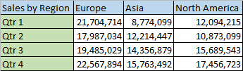
The Transpose feature will rearrange the table such that the Quarters are showing in the column headings and the Sales Regions can be seen on the left, like this:
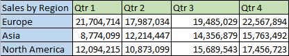
Note: If your data is in an Excel table, the Transpose feature won’t be available. You can convert the table to a range first, or you can use the TRANSPOSE function to rotate the rows and columns.
Here’s how to do it:
Select the range of data you want to rearrange, including any row or column labels, and press Ctrl+C.
Note: Ensure that you copy the data to do this, since using the Cut command or Ctrl+X won’t work.
Choose a new location in the worksheet where you want to paste the transposed table, ensuring that there is plenty of room to paste your data. The new table that you paste there will entirely overwrite any data / formatting that’s already there.
Right-click over the top-left cell of where you want to paste the transposed table, then choose Transpose  .
.
After rotating the data successfully, you can delete the original table and the data in the new table will remain intact.
Tips for transposing your data
If your data includes formulas, Excel automatically updates them to match the new placement. Verify these formulas use absolute references—if they don’t, you can switch between relative, absolute, and mixed references before you rotate the data.
If you want to rotate your data frequently to view it from different angles, consider creating a PivotTable so that you can quickly pivot your data by dragging fields from the Rows area to the Columns area (or vice versa) in the PivotTable Field List.
You can paste data as transposed data within your workbook. Transpose reorients the content of copied cells when pasting. Data in rows is pasted into columns and vice versa.
Here’s how you can transpose cell content:
Copy the cell range.
Select the empty cells where you want to paste the transposed data.
On the Home tab, click the Paste icon, and select Paste Transpose.
Need more help?
You can always ask an expert in the Excel Tech Community or get support in the Answers community.
Источник
How You Can Convert Rows to Columns or Columns to Rows in Excel Workbooks
Do you have some values arranged as rows in your workbook, and do you want to convert text in rows to columns in Excel like this?
In Excel, you can do this manually or automatically in multiple ways depending on your purpose. Read on to get all the details and choose the best solution for yourself.
How to convert rows into columns or columns to rows in Excel – the basic solution
The easiest way to convert rows to columns in Excel is via the Paste Transpose option. Here is how it looks:
- Select and copy the needed range
- Right-click on a cell where you want to convert rows to columns
- Select the Paste Transpose option to rotate rows to columns
![]()
As an alternative, you can use the Paste Special option and mark Transpose using its menu.
It works the same if you need to convert columns to rows in Excel.
This is the best way for a one-time conversion of small to medium numbers of rows both in the Excel desktop and online.
Can I convert multiple rows to columns in Excel from another workbook?
The method above will work well if you want to convert rows to columns in Excel between different workbooks using Excel desktop. You need to have both spreadsheets open and do the copying and pasting as described.
However, in Excel Online, this won’t work for different workbooks. The Paste Transpose option is not available.
Therefore, in this case, it’s better to use the TRANSPOSE function.
How to switch rows and columns in Excel in more efficient ways
To switch rows and columns in Excel automatically or dynamically, you can use one of these options:
- Excel TRANSPOSE function
- VBA macro
- Power Query
Let’s check out each of them in the example of a data range that we imported to Excel from a Google Sheets file using Coupler.io.
Coupler.io is an integration solution that synchronizes data between source and destination apps on a regular schedule. For example, you can set up an automatic data export from Google Sheets every day to your Excel workbook.
Check out all the available Excel integrations.
How to change row to column in Excel with TRANSPOSE
TRANSPOSE is the Excel function that allows you to switch rows and columns in Excel. Here is its syntax:
- array – an array of columns or rows to transpose
One of the main benefits of TRANSPOSE is that it links the converted columns/rows with the source rows/columns. So, if the values in the rows change, the same changes will be made in the converted columns.
TRANSPOSE formula to convert multiple rows to columns in Excel desktop
TRANSPOSE is an array formula, which means that you’ll need to select a number of cells in the columns that correspond to the number of cells in the rows to be converted and press Ctrl+Shift+Enter.
![]()
Fortunately, you don’t have to go through this procedure in Excel Online.
TRANSPOSE formula to rotate row to column in Excel Online
You can simply insert your TRANSPOSE formula in a cell and hit enter. The rows will be rotated to columns right away without any additional button combinations.
![]()
Excel TRANSPOSE multiple rows in a group to columns between different workbooks
We promised to demonstrate how you can use TRANSPOSE to rotate rows to columns between different workbooks. In Excel Online, you need to do the following:
- Copy a range of columns to rotate from one spreadsheet and paste it as a link to another spreadsheet.
- We need this URL path to use in the TRANSPOSE formula, so copy it.
- The URL path above is for a cell, not for an array. So, you’ll need to slightly update it to an array to use in your TRANSPOSE formula. Here is what it should look like:
![]()
You can follow the same logic for rotating rows to columns between workbooks in Excel desktop.
Are there other formulas to convert columns to rows in Excel?
TRANSPOSE is not the only function you can use to change rows to columns in Excel. A combination of INDIRECT and ADDRESS functions can be considered as an alternative, but the flow to convert rows to columns in Excel using this formula is much trickier. Let’s check it out in the following example.
How to convert text in columns to rows in Excel using INDIRECT+ADDRESS
If you have a set of columns with the first cell A1, the following formula will allow you to convert columns to rows in Excel.
But where are the rows, you may ask! Well, first you need to drag this formula down if you are converting multiple columns to rows. Then drag it to the right.
NOTE: This Excel formula only to convert data in columns to rows starting with A1 cell. If your columns start from another cell, check out the next section.
How to convert Excel data in columns to rows using INDIRECT+ADDRESS from other cells
To convert columns to rows in Excel with INDIRECT+ADDRESS formulas from not A1 cell only, use the following formula:
- first_cell – enter the first cell of your columns
Here is an example of how to convert Excel data in columns to rows:
Again, you’ll need to drag the formula down and to the right to populate the rest of the cells.
How to automatically convert rows to columns in Excel VBA
VBA is a superb option if you want to customize some function or functionality. However, this option is only code-based. Below we provide a script that allows you to change rows to columns in Excel automatically.
- Go to the Visual Basic Editor (VBE). Click Alt+F11 or you can go to the Developer tab => Visual Basic.
- In VBE, go to Insert => Module.
- Copy and paste the script into the window. You’ll find the script in the next section.
- Now you can close the VBE. Go to Developer => Macros and you’ll see your RowsToColumns macro. Click Run.
- You’ll be asked to select the array to rotate and the cell to insert the rotated columns.
- There you go!
VBA macro script to convert multiple rows to columns in Excel
Convert rows to column in Excel using Power Query
Power Query is another powerful tool available for Excel users. We wrote a separate Power Query Tutorial, so feel free to check it out.
Meanwhile, you can use Power Query to transpose rows to columns. To do this, go to the Data tab, and create a query from table.
- Then select a range of cells to convert rows to columns in Excel. Click OK to open the Power Query Editor.
- In the Power Query Editor, go to the Transform tab and click Transpose. The rows will be rotated to columns.
![]()
- If you want to keep the headers for your columns, click the Use First Row as Headers button.
- That’s it. You can Close & Load your dataset – the rows will be converted to columns.
Error message when trying to convert rows to columns in Excel
To wrap up with converting Excel data in columns to rows, let’s review the typical error messages you can face during the flow.
Overlap error
The overlap error occurs when you’re trying to paste the transposed range into the area of the copied range. Please avoid doing this.
Wrong data type error
You may see this #VALUE! error when you implement the TRANSPOSE formula in Excel desktop without pressing Ctrl+Shift+Enter.
Other errors may be caused by typos or other misprints in the formulas you use to convert groups of data from rows to columns in Excel. Always double-check the syntax before pressing Enter or Ctrl+Shift+Enter 🙂 . Good luck with your data!
Источник