
When you move or copy rows and columns, by default Excel moves or copies all data that they contain, including formulas and their resulting values, comments, cell formats, and hidden cells.
When you copy cells that contain a formula, the relative cell references are not adjusted. Therefore, the contents of cells and of any cells that point to them might display the #REF! error value. If that happens, you can adjust the references manually. For more information, see Detect errors in formulas.
You can use the Cut command or Copy command to move or copy selected cells, rows, and columns, but you can also move or copy them by using the mouse.
By default, Excel displays the Paste Options button. If you need to redisplay it, go to Advanced in Excel Options. For more information, see Advanced options.
-
Select the cell, row, or column that you want to move or copy.
-
Do one of the following:
-
To move rows or columns, on the Home tab, in the Clipboard group, click Cut
 or press CTRL+X.
 -
To copy rows or columns, on the Home tab, in the Clipboard group, click Copy
or press CTRL+C.
-
-
Right-click a row or column below or to the right of where you want to move or copy your selection, and then do one of the following:
-
When you are moving rows or columns, click Insert Cut Cells.
-
When you are copying rows or columns, click Insert Copied Cells.
Tip: To move or copy a selection to a different worksheet or workbook, click another worksheet tab or switch to another workbook, and then select the upper-left cell of the paste area.
-
 or press CTRL+X.
 or press CTRL+C.
Note: Excel displays an animated moving border around cells that were cut or copied. To cancel a moving border, press Esc.
By default, drag-and-drop editing is turned on so that you can use the mouse to move and copy cells.
-
Select the row or column that you want to move or copy.
-
Do one of the following:
-
Cut and replace
Point to the border of the selection. When the pointer becomes a move pointer, drag the rows or columns to another location. Excel warns you if you are going to replace a column. Press Cancel to avoid replacing. -
Copy and replace Hold down CTRL while you point to the border of the selection. When the pointer becomes a copy pointer
, drag the rows or columns to another location. Excel doesn’t warn you if you are going to replace a column. Press CTRL+Z if you don’t want to replace a row or column. -
Cut and insert Hold down SHIFT while you point to the border of the selection. When the pointer becomes a move pointer
, drag the rows or columns to another location. -
Copy and insert Hold down SHIFT and CTRL while you point to the border of the selection. When the pointer becomes a move pointer
, drag the rows or columns to another location.
Note: Make sure that you hold down CTRL or SHIFT during the drag-and-drop operation. If you release CTRL or SHIFT before you release the mouse button, you will move the rows or columns instead of copying them.
-
 , drag the rows or columns to another location. Excel warns you if you are going to replace a column. Press Cancel to avoid replacing.
 , drag the rows or columns to another location. Excel doesn’t warn you if you are going to replace a column. Press CTRL+Z if you don’t want to replace a row or column.
Note: You cannot move or copy nonadjacent rows and columns by using the mouse.
If some cells, rows, or columns on the worksheet are not displayed, you have the option of copying all cells or only the visible cells. For example, you can choose to copy only the displayed summary data on an outlined worksheet.
-
Select the row or column that you want to move or copy.
-
On the Home tab, in the Editing group, click Find & Select, and then click Go To Special.
-
Under Select, click Visible cells only, and then click OK.
-
On the Home tab, in the Clipboard group, click Copy
or press Ctrl+C. . -
Select the upper-left cell of the paste area.
Tip: To move or copy a selection to a different worksheet or workbook, click another worksheet tab or switch to another workbook, and then select the upper-left cell of the paste area.
-
On the Home tab, in the Clipboard group, click Paste
or press Ctrl+V.If you click the arrow below Paste
, you can choose from several paste options to apply to your selection.
 or press Ctrl+V.
Excel pastes the copied data into consecutive rows or columns. If the paste area contains hidden rows or columns, you might have to unhide the paste area to see all of the copied cells.
When you copy or paste hidden or filtered data to another application or another instance of Excel, only visible cells are copied.
-
Select the row or column that you want to move or copy.
-
On the Home tab, in the Clipboard group, click Copy
or press Ctrl+C. -
Select the upper-left cell of the paste area.
-
On the Home tab, in the Clipboard group, click the arrow below Paste
, and then click Paste Special. -
Select the Skip blanks check box.
-
Double-click the cell that contains the data that you want to move or copy. You can also edit and select cell data in the formula bar.
-
Select the row or column that you want to move or copy.
-
On the Home tab, in the Clipboard group, do one of the following:
-
To move the selection, click Cut
or press Ctrl+X. -
To copy the selection, click Copy
or press Ctrl+C.
-
-
In the cell, click where you want to paste the characters, or double-click another cell to move or copy the data.
-
On the Home tab, in the Clipboard group, click Paste
or press Ctrl+V. -
Press ENTER.
Note: When you double-click a cell or press F2 to edit the active cell, the arrow keys work only within that cell. To use the arrow keys to move to another cell, first press Enter to complete your editing changes to the active cell.
When you paste copied data, you can do any of the following:
-
Paste only the cell formatting, such as font color or fill color (and not the contents of the cells).
-
Convert any formulas in the cell to the calculated values without overwriting the existing formatting.
-
Paste only the formulas (and not the calculated values).
Procedure
-
Select the row or column that you want to move or copy.
-
On the Home tab, in the Clipboard group, click Copy
or press Ctrl+C.
-
Select the upper-left cell of the paste area or the cell where you want to paste the value, cell format, or formula.
-
On the Home tab, in the Clipboard group, click the arrow below Paste
, and then do one of the following:-
To paste values only, click Values.
-
To paste cell formats only, click Formatting.
-
To paste formulas only, click Formulas.
-
When you paste copied data, the pasted data uses the column width settings of the target cells. To correct the column widths so that they match the source cells, follow these steps.
-
Select the row or column that you want to move or copy.
-
On the Home tab, in the Clipboard group, do one of the following:
-
To move cells, click Cut
or press Ctrl+X. -
To copy cells, click Copy
or press Ctrl+C.
-
-
Select the upper-left cell of the paste area.
Tip: To move or copy a selection to a different worksheet or workbook, click another worksheet tab or switch to another workbook, and then select the upper-left cell of the paste area.
-
On the Home tab, in the Clipboard group, click the arrow under Paste
, and then click Keep Source Column Widths.
You can use the Cut command or Copy command to move or copy selected cells, rows, and columns, but you can also move or copy them by using the mouse.
-
Select the cell, row, or column that you want to move or copy.
-
Do one of the following:
-
To move rows or columns, on the Home tab, in the Clipboard group, click Cut
or press CTRL+X. -
To copy rows or columns, on the Home tab, in the Clipboard group, click Copy
or press CTRL+C.
-
-
Right-click a row or column below or to the right of where you want to move or copy your selection, and then do one of the following:
-
When you are moving rows or columns, click Insert Cut Cells.
-
When you are copying rows or columns, click Insert Copied Cells.
Tip: To move or copy a selection to a different worksheet or workbook, click another worksheet tab or switch to another workbook, and then select the upper-left cell of the paste area.
-
Note: Excel displays an animated moving border around cells that were cut or copied. To cancel a moving border, press Esc.
-
Select the row or column that you want to move or copy.
-
Do one of the following:
-
Cut and insert
Point to the border of the selection. When the pointer becomes a hand pointer, drag the row or column to another location -
Cut and replace Hold down SHIFT while you point to the border of the selection. When the pointer becomes a move pointer
, drag the row or column to another location. Excel warns you if you are going to replace a row or column. Press Cancel to avoid replacing. -
Copy and insert Hold down CTRL while you point to the border of the selection. When the pointer becomes a move pointer
, drag the row or column to another location. -
Copy and replace Hold down SHIFT and CTRL while you point to the border of the selection. When the pointer becomes a move pointer
, drag the row or column to another location. Excel warns you if you are going to replace a row or column. Press Cancel to avoid replacing.
Note: Make sure that you hold down CTRL or SHIFT during the drag-and-drop operation. If you release CTRL or SHIFT before you release the mouse button, you will move the rows or columns instead of copying them.
-
 , drag the row or column to another location
Note: You cannot move or copy nonadjacent rows and columns by using the mouse.
-
Double-click the cell that contains the data that you want to move or copy. You can also edit and select cell data in the formula bar.
-
Select the row or column that you want to move or copy.
-
On the Home tab, in the Clipboard group, do one of the following:
-
To move the selection, click Cut
or press Ctrl+X. -
To copy the selection, click Copy
or press Ctrl+C.
-
-
In the cell, click where you want to paste the characters, or double-click another cell to move or copy the data.
-
On the Home tab, in the Clipboard group, click Paste
or press Ctrl+V. -
Press ENTER.
Note: When you double-click a cell or press F2 to edit the active cell, the arrow keys work only within that cell. To use the arrow keys to move to another cell, first press Enter to complete your editing changes to the active cell.
When you paste copied data, you can do any of the following:
-
Paste only the cell formatting, such as font color or fill color (and not the contents of the cells).
-
Convert any formulas in the cell to the calculated values without overwriting the existing formatting.
-
Paste only the formulas (and not the calculated values).
Procedure
-
Select the row or column that you want to move or copy.
-
On the Home tab, in the Clipboard group, click Copy
or press Ctrl+C.
-
Select the upper-left cell of the paste area or the cell where you want to paste the value, cell format, or formula.
-
On the Home tab, in the Clipboard group, click the arrow below Paste
, and then do one of the following:-
To paste values only, click Paste Values.
-
To paste cell formats only, click Paste Formatting.
-
To paste formulas only, click Paste Formulas.
-
You can move or copy selected cells, rows, and columns by using the mouse and Transpose.
-
Select the cells or range of cells that you want to move or copy.
-
Point to the border of the cell or range that you selected.
-
When the pointer becomes a
, do one of the following:
 , do one of the following:
|
To |
Do this |
|---|---|
|
Move cells |
Drag the cells to another location. |
|
Copy cells |
Hold down OPTION and drag the cells to another location. |
Note: When you drag or paste cells to a new location, if there is pre-existing data in that location, Excel will overwrite the original data.
-
Select the rows or columns that you want to move or copy.
-
Point to the border of the cell or range that you selected.
-
When the pointer becomes a
, do one of the following:
|
To |
Do this |
|---|---|
|
Move rows or columns |
Drag the rows or columns to another location. |
|
Copy rows or columns |
Hold down OPTION and drag the rows or columns to another location. |
|
Move or copy data between existing rows or columns |
Hold down SHIFT and drag your row or column between existing rows or columns. Excel makes space for the new row or column. |
-
Copy the rows or columns that you want to transpose.
-
Select the destination cell (the first cell of the row or column into which you want to paste your data) for the rows or columns that you are transposing.
-
On the Home tab, under Edit, click the arrow next to Paste, and then click Transpose.
Note: Columns and rows cannot overlap. For example, if you select values in Column C, and try to paste them into a row that overlaps Column C, Excel displays an error message. The destination area of a pasted column or row must be outside the original values.
See also
Insert or delete cells, rows, columns
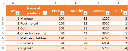
While working on a worksheet that has numerous rows of data, you may have to reorder the row and columns every now and then. Whether it’s a simple mistake or the data is not at the right spot or you simply need to rearrange the data, then you have to move rows or columns in Excel.
If you work with Excel tables a lot, it’s important to know how to move rows or columns in Excel. There are three ways to move rows or columns in Excel, including the drag method using the mouse, cut and paste, and rearrange rows using the Data Sort feature. In this tutorial, we will cover all three methods one by one.
Move a Row/Column by Dragging and Dropping in Excel
The drag and drop method is the easiest way to quickly move rows in a dataset. But dragging rows in Excel is a bit more complex than you realize. There are three ways you can drag-and-drop rows in Excel, including drag and replace, drag and copy, and drag and move.
Drag and Replace Row
The first method is a simple drag and drop but the moving row will replace the destination row.
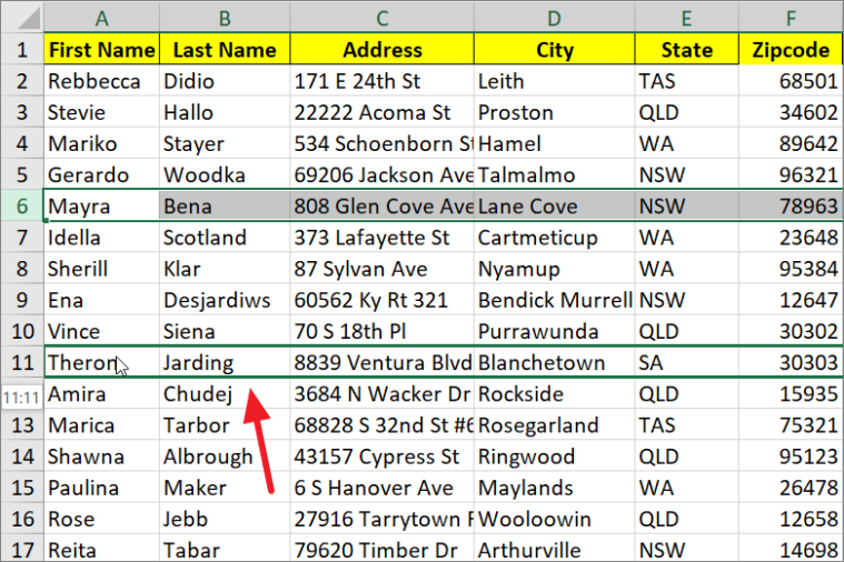
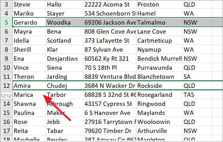
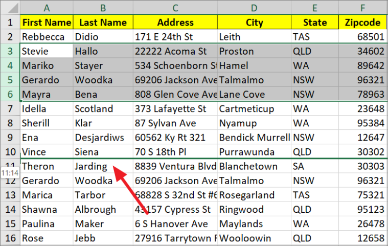
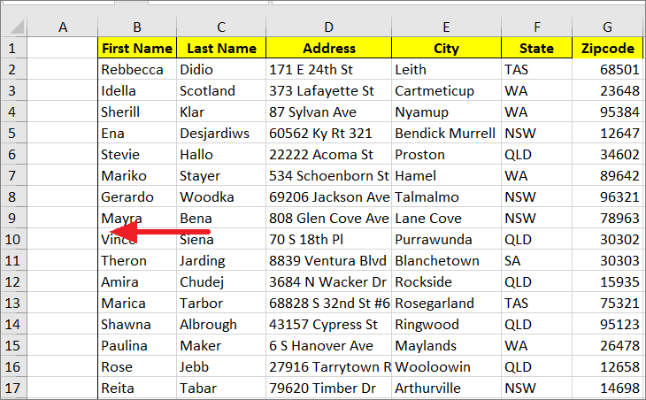
First, select the row (or contiguous rows) that you want to move. You can select an entire row by simply clicking the row number or clicking on any cell in the row and pressing Shift+Spacebar. Here, we’re selecting row 6.
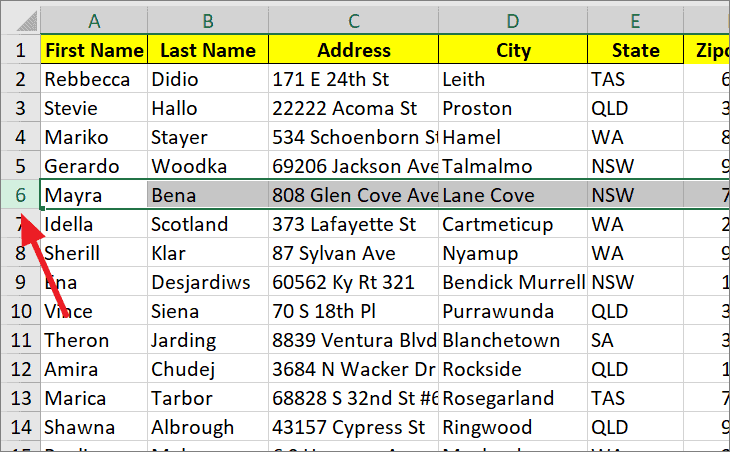
After selecting the row, move your cursor to the edge of the selection (either top or bottom). You should see your cursor change to a move pointer ![]() (cross with the arrows).
(cross with the arrows).
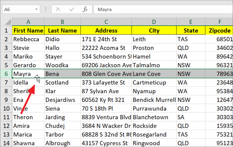
Now, hold down the left mouse click, and drag it (top or bottom) to the desired location where you want to move the row. While you’re dragging the row, it will highlight the current row in a green border. In the example, we’re dragging row 6 to row 11.
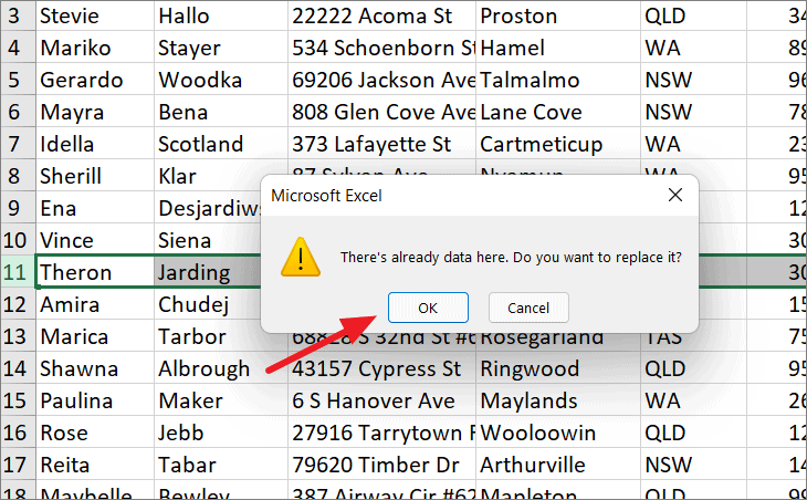
Then, release the left mouse button and you will see a pop-up asking “There’s already data here. Do you want to replace it?”. Click ‘OK’ to replace row 11 with the data of row 6.
But, when you move your row to an empty row, Excel won’t show you this pop-up, it will simply move the data to the empty row.
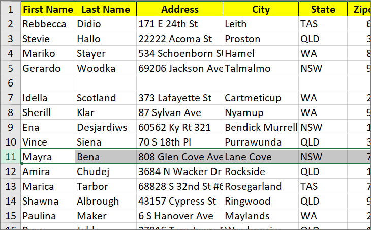
In the below screenshot, you can see that row 11 is now replaced with row 6.
Drag and Move/Swap Row
You can quickly move or swap a row without overwriting the existing row by holding the Shift key when dragging the selected row(s).
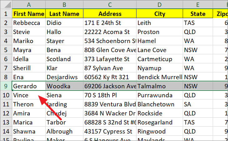
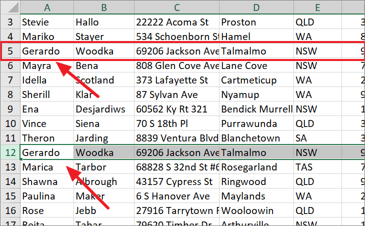
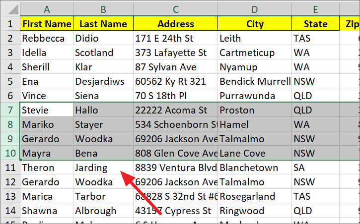
Select your row (or contiguous row) that you want to move the same you did in the above section. Here, we’re selecting row 5.
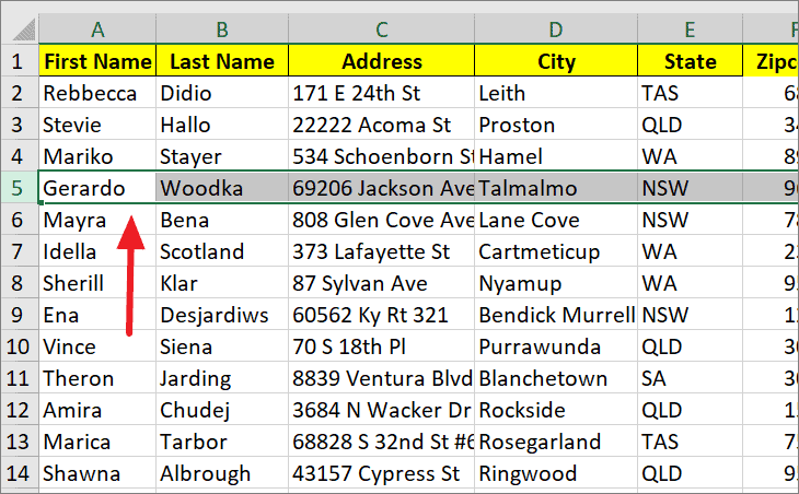
Next, press and hold the Shift key on the keyboard, move your cursor to the edge of the selection (either top or bottom). When your cursor turns to a move pointer ![]() (cross with the arrow), click on the edge (with left mouse button), and drag the row to the new location.
(cross with the arrow), click on the edge (with left mouse button), and drag the row to the new location.
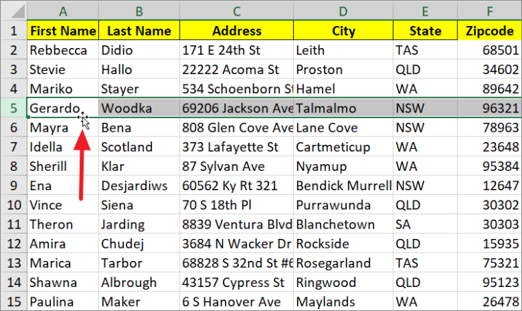
When you drag your cursor across the rows, you would see a bold green line at the edge of the row indicating where the new row will appear. Once you’ve found the right location for the row, release the mouse click and the Shift key. Here, we want to move row 5 to between rows 9 and 10.
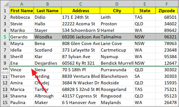
Once the mouse button is released, row 5 is moved to row 9, and the original row 9 automatically moves up.
This method basically cuts the row and then inserts them to the new location (where you release the mouse button) without overwriting the existing row.
Drag and Copy Row
If you want to copy the row to the new location then simply press the Ctrl key while dragging the row to the new location. This method also replaces the destination row but it keeps the existing row (moving row) in place.
Select the row(s) you want to move the same way we did in the previous sections. Here, we’re selecting row 5.
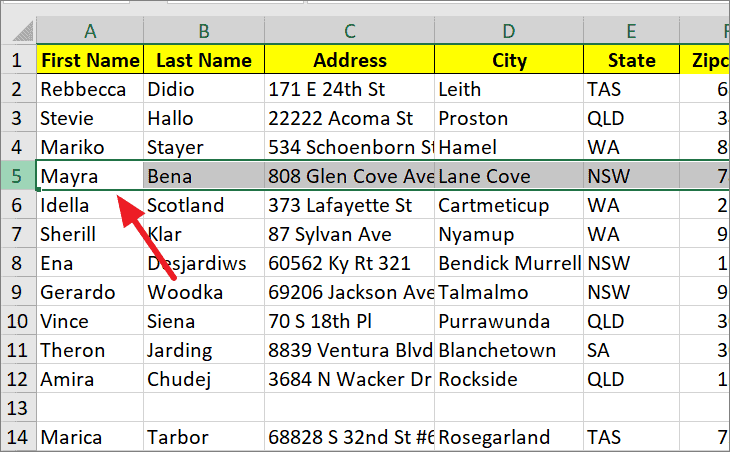
This time, press and hold the Ctrl key on the keyboard, and drag the row to your desired location using the move pointer. Once you’ve found the right spot for the row, release the mouse click and the Ctrl key. Here, we’re releasing the mouse click at row 12.
Upon releasing the buttons, the 5th-row data replaces the 12th-row data but the 5th-row remains as the original data. Also, there is no pop-up dialog box asking whether to overwrite the data or not.
Move Multiple Rows At A Time by Dragging
You can also move multiple rows at a time using any of the same above methods. However, you can only move contiguous/adjacent rows and you cannot move non-contiguous rows by dragging.
First, select the multiple rows you want to move. You can select the entire multiple rows by clicking and dragging over the row numbers to the left. Alternatively, click on the first or last row header you want to select, press and hold the Shift key and use the arrow keys up or down to select multiple rows. In the example below, we’re selecting from rows 3 to 6.
Now, click on the edge of the selection, and drag the rows to the new location. You can simply drag, drag while holding the Shift key, or drag while holding the Ctrl key to move the rows.
In the example, we’re dragging the rows while holding the Shift key until the bottom line of row 10.
Now, rows 3 to 6 are moved to the location of rows 7 to 10, and the original rows from 7 to 10 are moved/shifted up.
Move Column using Mouse Drag
You can move columns (or contiguous columns) by following the same steps you did for the rows.
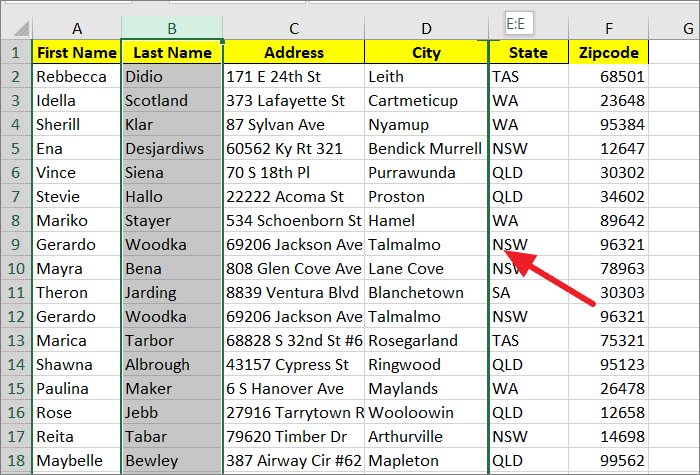
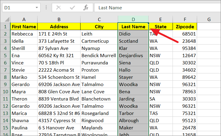
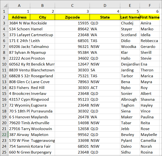
First, select the column (or adjacent columns) that you want to move. You can select an entire column by clicking the column header (column letter) at the top or pressing the Ctrl+Spacebar shortcut keys. In the example, we want column B (Last Name) to come after column D (City), so we’re highlighting column B.
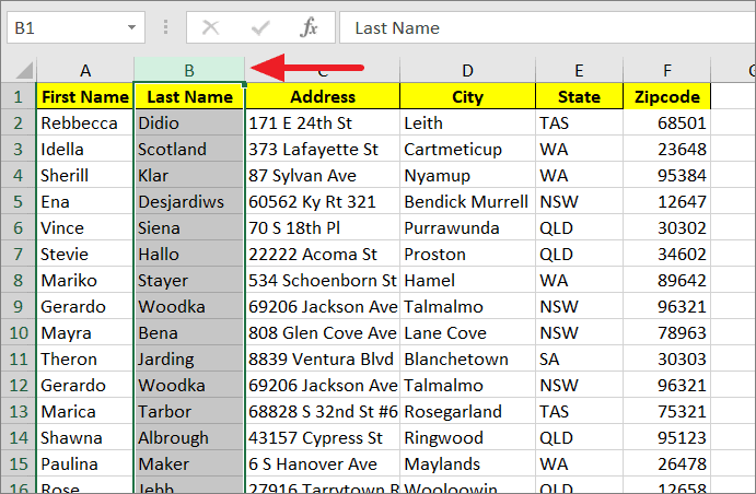
Then, drag the column using Shift + left mouse click and release the mouse button and Shift key when you see the green bold line at the edge between column D and column E.
You can also simply drag the column or hold the Ctrl key while dragging the column to move and replace the existing column.
As you can see column B is moved to the location indicated by the bold green border and the original column D (City) is shifted to the left.
Move a Row/Column in Excel With Cut and Paste
Another easiest and well-known method for moving rows in Excel is by cutting and pasting the row of cells from one location to another. You can easily cut and paste rows using shortcut keys or mouse right-click. This method is much more simple and straightforward than the previous method. Let’s see how to move rows using the cut and paste method.
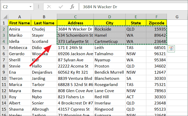
First, select the row (or contiguous rows ) as we did in the previous sections. You can either select an entire row or a range of cells in a row. Then, press the Ctrl+X (Command+X on Mac computer) on your keyboard to cut the selected row from its current location. Alternatively, you can right-click on the selected cell and select ‘Cut’.
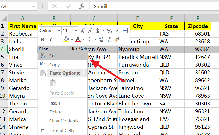
Once you did that, you will see the marching ants effects (moving border of dots) around the row to show it has been cut. In the below example, row 4 is cut.
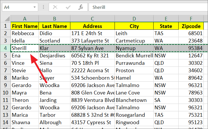
Next, select the desired destination row where you want to paste the cut row. If you moving an entire row, make sure to select the entire destination row by clicking the row number before pasting. Here, we’re selecting row 8.
Then, press the Ctrl+V shortcut keys to paste the row or right-click the destination row and click on the ‘Paste’ icon from the context menu.
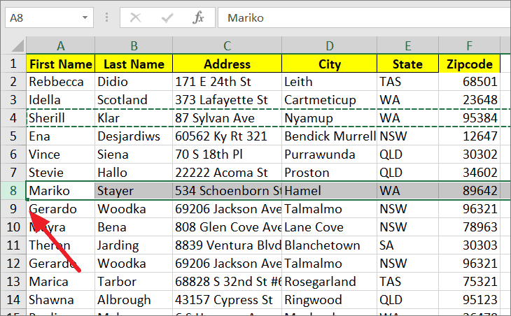
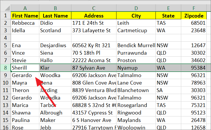
When you use this method to move rows, it will overwrite the existing row. As you can, the data of row 8 is replaced with the data of row 4 in the below screenshot.
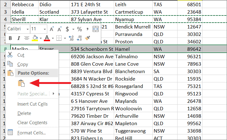
If you don’t want to replace the existing row while moving the selected row, you can use the ‘Insert Cut Cells’ option instead of the simple ‘Paste’ option. Here’s how you do that:
Select the row you want to move, and right-click and select ‘Cut’ or press Ctrl+X. Then, select the row before which you want to insert the cut row, right-click on it and choose ‘Insert Cut Cells’ from the context menu. Alternatively, you can press the Ctrl key + Plus sign (+) key on the numeric keypad to insert the cut row.
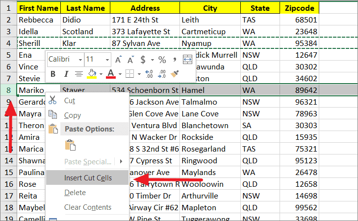
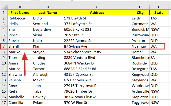
As you can see here, row 4 is inserted above the selected row, and the original row 7 is moved up.
If you want to copy the row rather than cut it, then instead of Ctrl+X, press Ctrl+C to copy the row and press Ctrl+V paste it. You can move columns using the cut and paste method by following these same instructions.
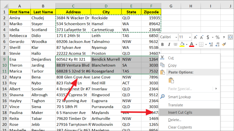
You can also cut a range of cells in a single row or multiple adjacent rows (contiguous rows) instead of entire rows and insert (or paste) them in another location using the above method. For example, we’re cutting C2:F4. Remember, if you are selecting multiple rows in the range, the rows must be adjacent rows.
Then, we are pasting the cut rows in the range C9:F11 using the ‘Insert Cut Cells’ option from the right-click menu.
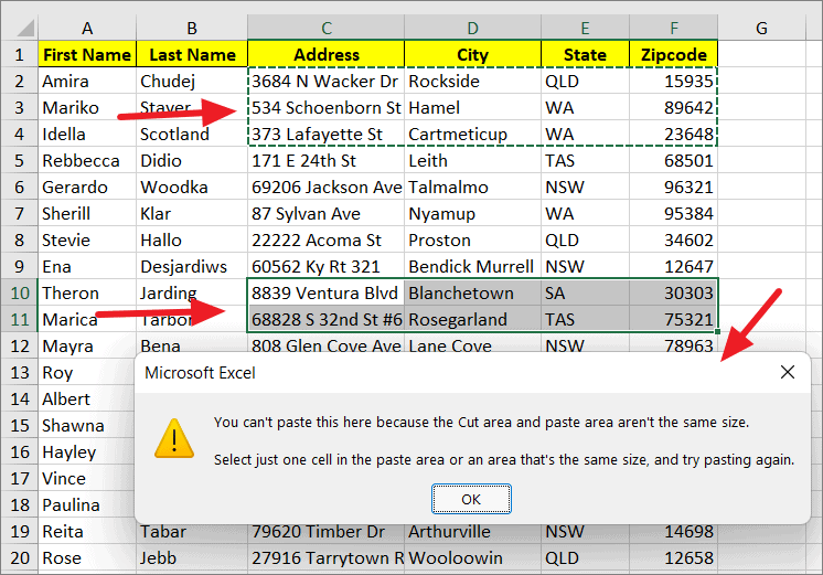
Also, when you are moving rows, the cut area and paste area must be the same size, otherwise, you would get an error when you try to paste the cut row. For example, if you cut rows C2:F4 and try to paste it in the smaller range C10:F11 using the normal paste (Ctrl+V) method, you would see the following error.
Move Rows Using a Data Sort Feature in Excel
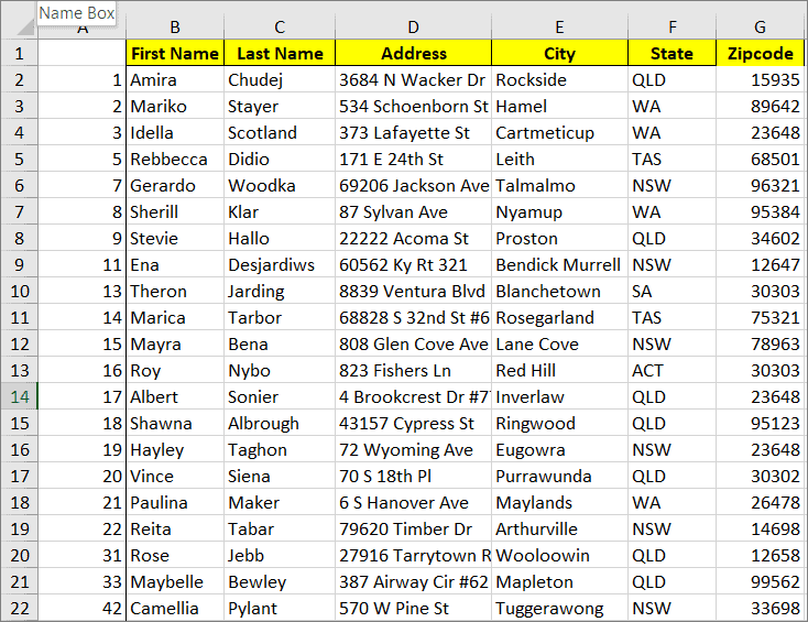
Moving rows with the data Sort features may require few more steps than the previous methods, but it is certainly not the difficult method to move rows or columns in Excel. Also, the data sort method comes with an advantage, you can change the order of all rows in one move that includes non-continuous rows as well. This method is certainly useful when it comes to rearranging numerous rows in a large spreadsheet. Follow these steps to move rows using a data sort:
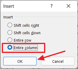
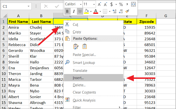
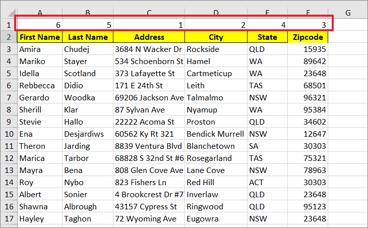
First, you need to add a column to the left-most side of your spreadsheet (column A). To do this, right-click on any cell in the first column and select the ‘Insert’ option from the context menu.
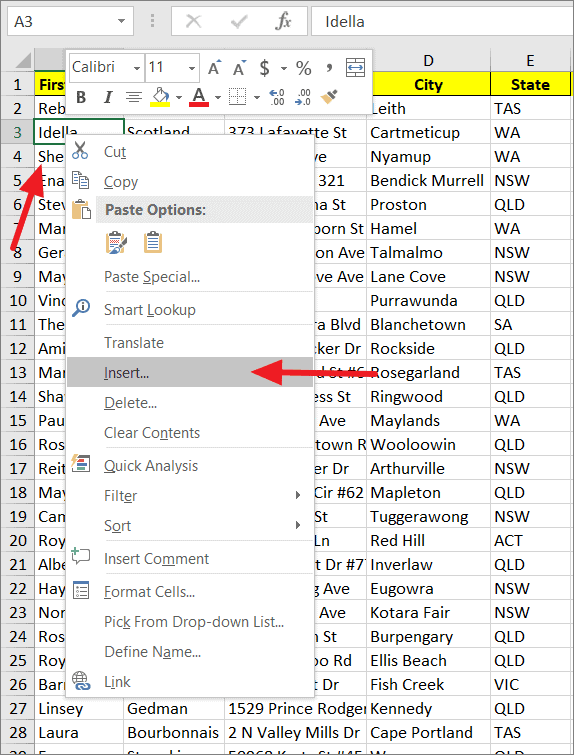
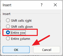
In the Insert pop-up box, select ‘Entire column’ and click ‘OK’.
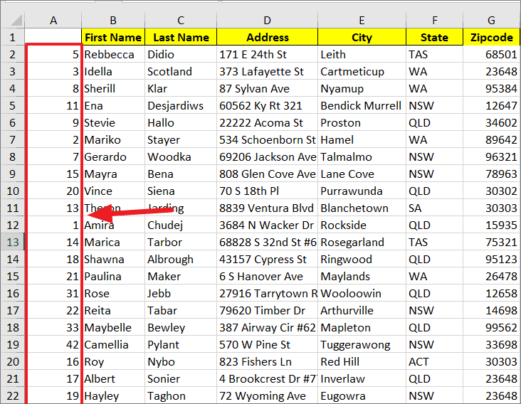
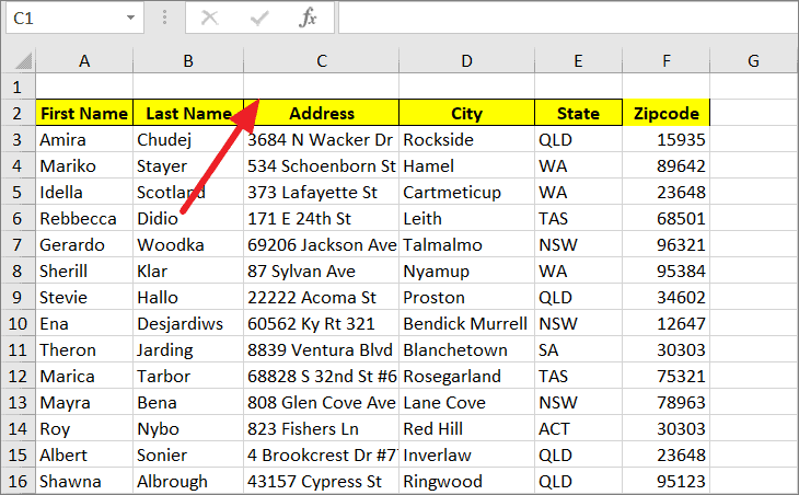
A new column has been inserted to the left-most side of your data set. This column must be the first column of your spreadsheet (i.e. column A).
Now, number the rows in the order you want them to appear in your spreadsheet by adding numbers in the first column as shown below.
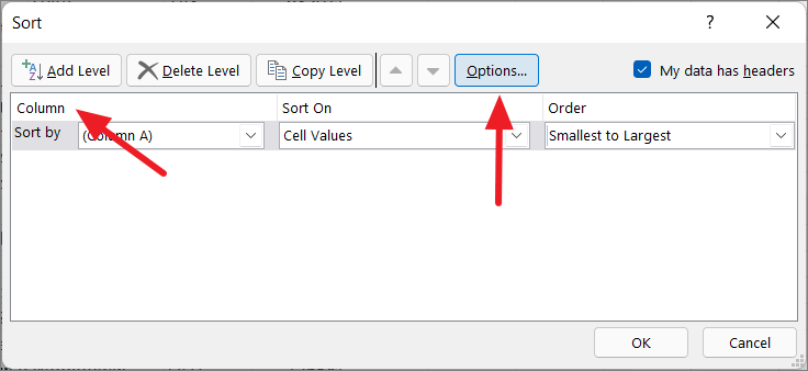
Next, select all the data in the dataset that you want to reorganize. Then, go to the ‘Data’ tab in the Ribbon, and click the ‘Sort’ button in the Sort & Filter group.
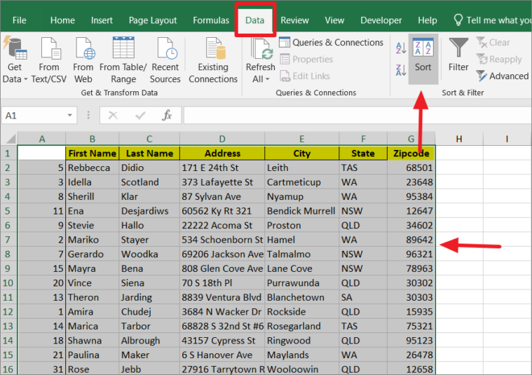
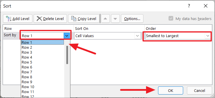
You need to sort the dataset by the numbers in Column A. So, in the Sort dialog box, make sure the sorting is set to ‘Column’ above the ‘Sort by’ drop-down. If not, click the ‘Options’ button at the top.
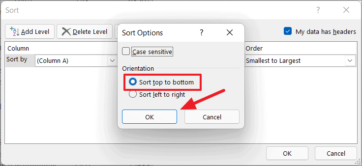
Then, in the Sort Options pop-up dialog, select ‘Sort top to bottom’ and click ‘OK’.
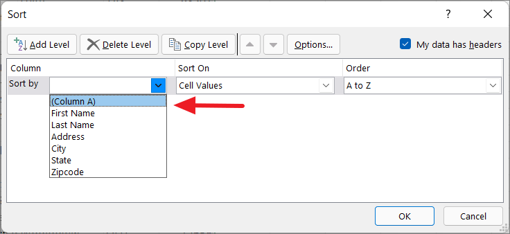
Now, you’ll be back on the Sort dialog window. Here, select ‘Column A’ (or title of your first column) in Sort By drop-down menu.
Then, make sure the ‘Order’ drop-down is set to ‘Smallest to Largest’ and click ‘OK’.
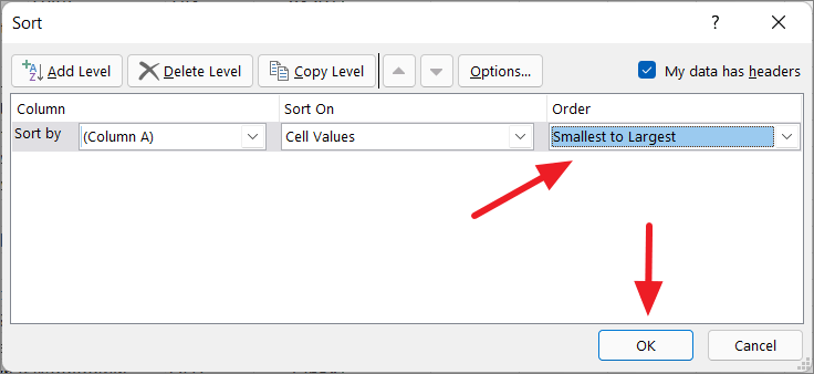
This will close the Sort dialog box and take you back to your spreadsheet, where you’ll find that the rows have been rearranged according to the numbers you listed in that first column. Now, select the first column, right-click and select ‘Delete’ to remove it.
Move Columns Using a Data Sort
The process of moving columns using data sort is essentially the same as the moving rows, with a only few different steps. Follow these steps to move columns using data sort.
To move columns, you need to add a row instead of a column to the top of your dataset (Row 1). To do this, right-click on any cell in the first row and select the ‘Insert’ option from the context menu.
In the Insert dialog box, select ‘Entire row’ this time and click ‘OK’.
A new row will be inserted to the top of your spreadsheet, above all rows of data.
Now, number the columns in the order you want them to appear in your worksheet by adding numbers in the first row as shown below.
Next, select all the data in the dataset that you want to change the order of. Then, switch to the ‘Data’ tab in the Ribbon, and click the ‘Sort’ in the Sort & Filter group.
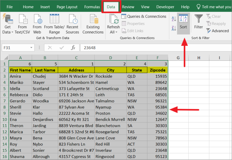
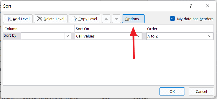
Now, you need to sort columns by the numbers in the first row. In the Sort dialog box, you need to set sorting to ‘Row’ instead of the column above the ‘Sort by’ drop-down. To do that, click the ‘Options’ button.
In the Sort Options pop-up dialog box, select ‘Sort left to right’ and click ‘OK’.
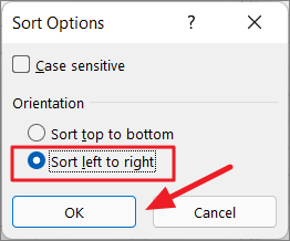
Back in the Sort dialog window, select ‘Row 1’ in Sort By drop-down menu and ‘Smallest to Largest’ in the Order drop-down. Then, click ‘OK’.
This will sort (move) the columns based on the numbers you listed in that first row as shown below. Now, all you have to do is select the first row and delete it.
Now, you know everything about moving rows as well as columns in Excel.
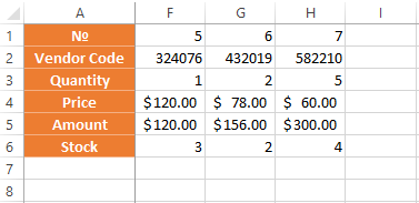
The Microsoft Excel program is designed not only to enter data into the table conveniently and edit it as you need it, but also to view large blocks of information. Most people using PCs work with it constantly.
The columns and rows names can be significantly removed from the cells with which the user is working at this time. Scrolling the page to see the name of the document is not comfortable for any user. Therefore, the Tabular Processor has possibilities to fix certain areas.
Locking a row in Excel while scrolling
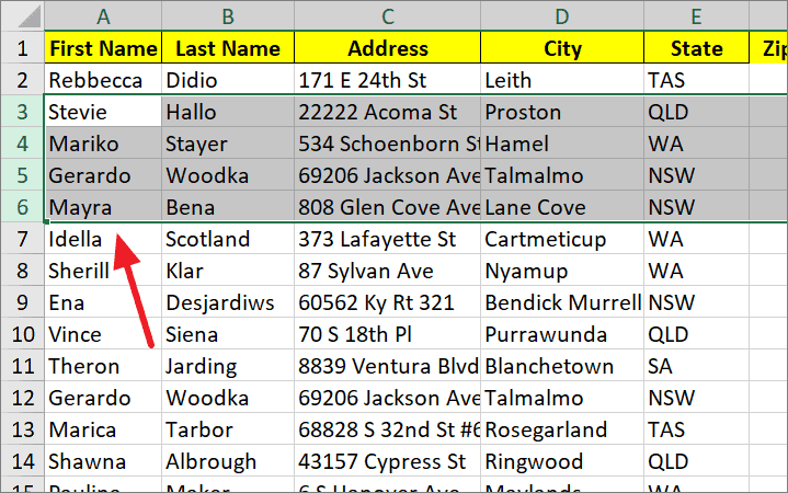
Usually an Excel table has one cap. Meanwhile, this document can have up to thousands of rows. Working with multipage table blocks is inconvenient when column names are not visible. Scrolling the page to its beginning to return to the correct cell is absolutely irrational. To make the cap visible when scrolling, fix the top row of the Excel table, following these actions:
- Create the needed table and fill it with the data.
- Make any of the cells active. Go to the “VIEW” tab using the tool “Freeze Panes”.
- In the menu select the “Freeze Top Row” functions.
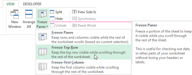
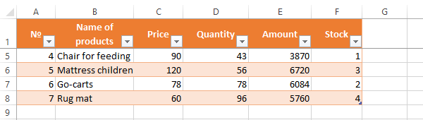
You will get a delimiting line under the top line. Now when you scroll vertically the table cap will be always visible.
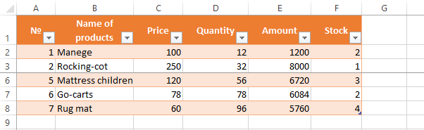
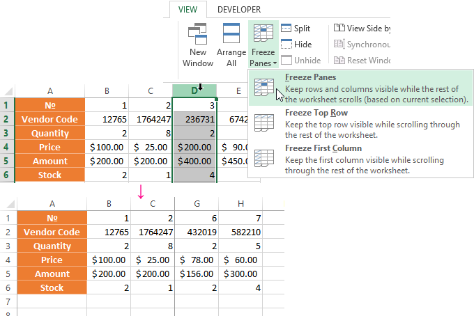
Locking several rows in Excel while scrolling
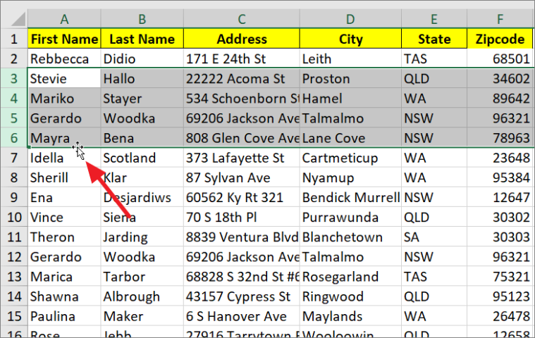
Let us suppose, a user needs to fix not only the cap. For instance, another row or even a couple of rows must be fixed when scrolling the document. Doing it is possible and easy, when you follow these steps:
- Select any cell under the line, which we will fix. This action will help Excel to “understand”, which area should be fixed;
- Now select the “Freeze Panes” tool.
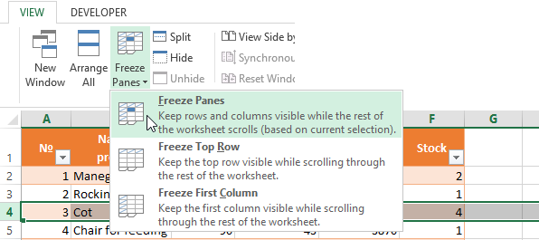
When you perform horizontal and vertical scrolling, the cap and the top row of the table remain fixed. Thus, you can fix two, three, four and more rows.
Note: This method works for 2007 and 2010 Excel versions. In earlier versions the “Lock areas” tool is located in the “Window” menu on the main page. There you must always (!) activate the cell under the freeze row.
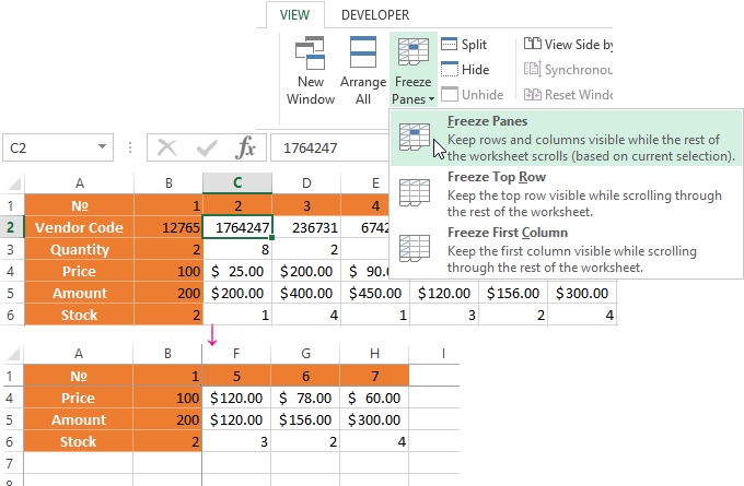
Freezing columns in Excel
For instance, the information in the table has a horizontal direction. It is not concentrated in columns, but located in rows. For his comfort, the user must freeze the first column, containing the lines’ names in horizontal scrolling.
- Select any cell of the chosen table so that Excel understands with what data it will work. Pin the first column in the menu you will see..
- Now, when the document is scrolled to the right horizontally, the needed column will be fixed.
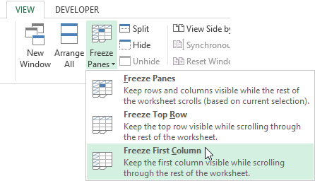
To freeze several columns, select the cell at the page bottom (to the right from the fixed column). Pick the “Freeze Panes” button.
How to freeze the row and column in Excel
You have a task – to freeze the selected area, which contains two columns and two rows.
Make a cell at the intersection of the fixed rows and columns active. However, the cell must be not placed in the fixed area. It should have the position right under the required lines (to the right of the required columns). Pick the first option in Excel Locking Areas. The photo shows that when scrolling, the selected areas remain at the same place.
Removing a fixed area in Excel
After fixing a row or a column of the table the button deleting all pivot tables becomes available.
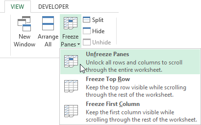
After clicking – «Unfreeze Panes», all the locked areas of the worksheet become unlocked.