Excel ribbon add in - Word и Excel - помощь в работе с программами

This Excel tutorial explains how to add Excel Add-in in Ribbon.

You may also want to read:

Writing your first Excel Macro by recording Macro

Why use Excel Add-in

After you have created a Macro (Sub Procedure), you may want to distribute it for users to use. You can simply add the VBA code in the Module of a Workbook and then distribute the Workbook, but the problem is that the Macro cannot be used in other Workbook.

Depending on the situation, you may want to distribute a Macro is through Add-in. Add-in is a file with extension .xla (for Excel 2003 and older version) and .xlam (for Excel 2007 and newer version) where users can use the Macro in any Workbook in his workstation. The Add-in itself is stored in the local drive of the receiver, it is not stored in a Workbook. If you have used Functions from Analysis ToolPak before, you realize that if you send the Workbook that used the Function (such as MRound, Networkdays) to others who do not have the Add-in, the formula will fail once refreshed.

To summarize, if your Macro is only for use in particular Workbook, you don’t have to use Add-in. If not, create an Add-in.

After creating an Excel Add-in, send the Add-in to users, then install the add-in.

In order to facilitate users to locate and run the Macro, I highly recommend to add the Macro in Ribbon.

In the following demonstration, I will use a real example where I create several Macro for users to validate data, such as data formatting and conflicting values.

Assume that you have already created several Sub Procedure in the Module of a Workbook. You should check carefully that “ThisWorkbook” refers to the Add-in Workbook, not the ActiveWorkbook. Change from “ThisWorkbook” to “ActiveWorkbook” if needed.

The next step is to tell Excel to create a ribbon.

In VBE (Alt+F11), double click on ThisWorkBook under VBA Project of the Add-In, we need to add two Events here:

Workbook.AddinInstall Event – Triggered when users install the Add-in. We are going to tell Excel to add ribbon here.

Workbook.AddinUninstall Event – Triggered when users uninstall the Add-in. We are going to tell Excel to remove ribbon here.

Insert the following code in ThisWorkbook

Private Sub Workbook_AddinInstall()
    With Application.CommandBars("Formatting").Controls.Add
        .Caption = "Identify incorrect Date format"  'The button caption
        .Style = msoButtonCaption
        .OnAction = "checkDateText"  'The Macro name you want to trigger
    End With
End Sub

Private Sub Workbook_AddinUninstall()
    On Error Resume Next
        Application.CommandBars("Formatting").Controls("Identify incorrect Date format").Delete
    On Error GoTo 0
End Sub

The above code adds a button called Identify incorrect Date format. If you want to add more, copy the code and change the Caption and OnAction parameters.

Save Excel Add-In

Save the Workbook as you would normally save it, except that you save it as xlam file type for Add-In. Name the file as checking P2 template.

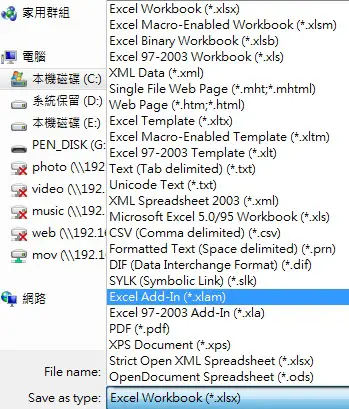
The xlam file icon looks like Excel, you can send this file for users to install.

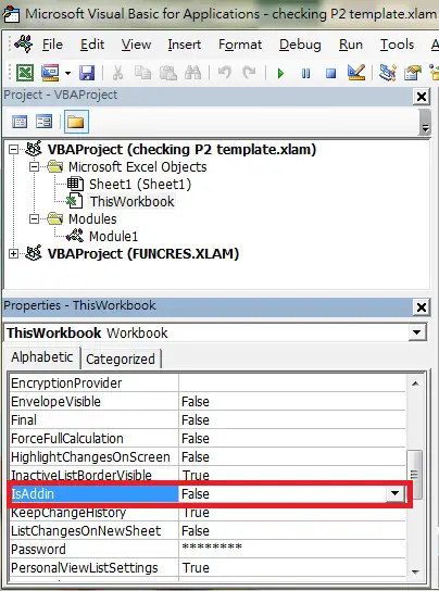
After you have saved the file as .xlam, all worksheets are hidden.

To change it back to a normal worksheet, change the IsAddin Property of ThisWorkbook to False.

Install Excel Add-in (User)

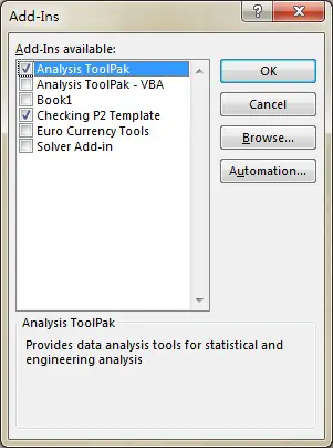
Navigate to Developer tab > Add-Ins, browse the Add-In location to add.

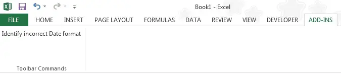
Now a tab called ADD-INS is added, under which is the button “Identify incorrect Date format”

If you have many items, you can group items by different CommandBars as below.

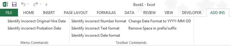
In the above example, I grouped them by Formatting / Worksheet Menu Bar

    With Application.CommandBars("Formatting").Controls.Add
        .Caption = "Remove Space in prefix/suffix"
        .Style = msoButtonCaption
        .OnAction = "checkSpace"
    End With 
        
    With Application.CommandBars("Worksheet Menu Bar").Controls.Add
        .Caption = "Identify incorrect Original Hire Date"
        .Style = msoButtonCaption
        .OnAction = "chk_Original_Hire_Dt"
    End With

Remove Excel Add-in

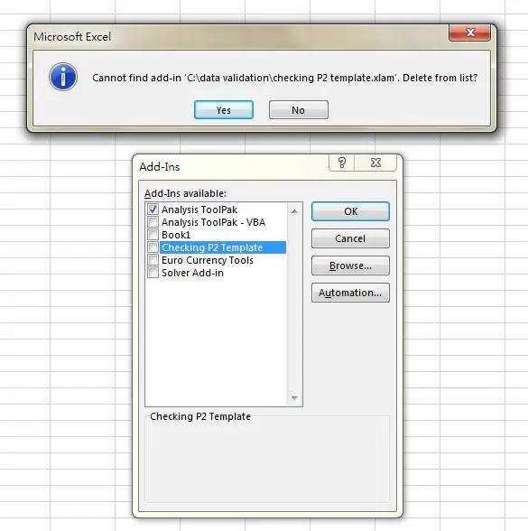
When you uncheck (uninstall) the box “Check P2 Template”, the option is still there.

If you want to completely remove the option from the Add-Ins box

1) Uncheck the Add-in

2) Close the workbook

3) Delete / Move the Add-Ins in your local drive

4) Open Excel, check the option of removed Add-in, then click on Yes to delete

http://sitestory.dk/excel_vba/my_menu.htm

Источник

Step by steph how to easily develope an Excel addin for your company

One of the most prosperous skills I have picked up over the years as a financial analyst has been the ability to create custom Excel add-ins specific to my department and company’s needs. This one skill I have been able to provide to my company has saved numerous people time, frustration, and money. While it took me well over a year to teach myself how to create top-notch add-ins, I want to let you in on a little secret….it’s really NOT THAT HARD! And today I want to share with you just how easy it can be to build an Excel add-in that looks amazing and will provide tremendous value to your company as well as to your professional career.

My First Excel Add-in Logo

JUST LAUNCHED!

Check out the My First Add-in template + Online Course which includes templates with many more Ribbon capabilities than the ones available in this article (includes Excel/PowerPoint/Word versions) and also a 6 module online video course to teach you how to customize the Ribbon outside of the template.

In this article, I will walk you through 5 simple steps:

Step 1: Download my free template (I have done all the difficult, nerdy stuff for you in this file)
Step 2: Link your macros and macro descriptions to the Ribbon buttons
Step 3: Test your buttons and make sure they work
Step 4: Choose the icons you want to display (Microsoft provides thousands for free!)
Step 5: Save your template as an add-in file and install/share

And Look What You Can Create!

Step 1: Download The Template

I went ahead and did all the tricky stuff for you and set up a template to give you a great head start. You can download this template by clicking the button below. This will allow you to skip all the difficult Ribbon coding.

After you’ve dowloaded the file, open it up in Microsoft Excel and move on to Step 2!

Step 2: Link Your Macros

Once you’ve opened your brand spanking new Excel Ribbon template, let’s dig into the VBA and link all your macro code snippets so they can be triggered by your Ribbon buttons. I am going to run through an example where I want to create a ribbon with just one macro button. Before we begin, make sure you have the file open and are looking at the Visual Basic Editor (shortcut key Alt + F11).

1. Hide Unused Groups & Buttons

Since I only want to create an add-in with one button and the template holds 50 buttons, I am going to want to hide the other 49 buttons. To do this, I need to navigate to the RibbonSetup module and then down to the GetVisible subroutine. You should see a Case statement that goes through each button name (ie myButton#) and tells the Ribbon whether to show the button (True) or hide it (False). Since I only want one button shown in this example, I’m going to make only the first button (myButton1) have a value of True.

Since the buttons are sectioned off into groups, I can just make the entire group not visible by modifying the Case Statements dealing with group IDs. In the example below I show GroupB not being visible.

2. Add Your Macro Code

Next, let’s add our macro code. I’m just going to use a simple piece of code that does the PasteSpecial command «Pastes Values Only» with the data currently copied to the clipboard.

Navigate to the Macros module and paste in your macro code.
Go back to the RibbonSetup module and scroll to the RunMacro subroutine
Add the macro name to the corresponding button name (overwriting the DummyMacro name)

3. Add A Screentip For Your Macros

A great way to help your users or yourself remember what a button does is to include a Screentip. A Screentip is a brief description that reminds the user what a button does while hovering over it. You see Screentips all the time in the normal Ribbon tabs, but you may have never noticed them. Go ahead and hover over a button on your Home tab and you’ll see some examples.

4. Add Your Tab, Group, & Button Names To The Ribbon UI

To finish off this section we are going to go down to the GetLabel subroutine within the RibbonSetup module. Similar to adding a Screentip, you can add a custom label via this macro that will display beneath your button on the Ribbon.

For this example, let’s call our Tab «Company», our group «PasteSpecial», and the button «Paste Values». As shown below, all we need to do is navigate to the GetLabel subroutine and modify the Labeling variable value to equal the text value we want to be displayed on the Ribbon tab.

At this point, we have linked our macro to a button, we’ve labeled the button, and provided a screentip so our users know what the button does. The major setup pieces are complete. Let’s move on to step 3!

Step 3: Test Your Buttons

This is a brief step but a very important one. After you have linked all your macros to the buttons on your Ribbon, you will want to save your file and close out of it. Re-open the file and see if all your setting tweaks actually flowed into the Macros tab (or in this example the Company tab). Also, start testing your macros to make sure they are all linked to the proper buttons and running as expected.

Step 4: Choose Your Icons

Next, is one of my favorite steps when designing a new add-in, picking out the icons! You might be wondering, how much money am I going to have to spend to get some nice looking icons for my add-in? Well lucky for us, Microsoft has been gracious enough to give everyone complete access to all of their fancy icons used throughout the Office Suite.

So how do we get these awesome icons? Well, remember all that work I did for you to create your handy starting point template? You don’t have to worry about finding the icons at all. All you need to do is tell Microsoft which icons to use by typing out their name in your VBA code. Just navigate to the GetImage subroutine and enter in the icon name with the respective button line. Since our example macro deals with pasting, I am going to use the PasteValues icon.

How Do You Get The Icon Names?

There are a few resources out there that have the Ribbon icon names, but I personally prefer the Excel file Microsoft created called Office 2007 Icons Gallery. This file displays all the icon images in 9 galleries up in the Developer tab of the Ribbon. If you hover over an image, the image’s name will appear in the ScreenTip box. You will need to copy this name verbatim (it is case sensitive!) and add it into the VBA macro called GetImage(), in the respective «case» section. Below is how I found the Page Break icon name.

Let me say it again: the icon name IS CASE SENSITIVE! So make sure you capitalize the correct characters.

How Do You Change The Icon Size?

As you may have noticed when you first opened up the template file, not all the icons are the same size. There are two available sizes that Microsoft allows you to make your icons (large or small). The size of what your icons will be is completely up to you. You may want to make important or heavily used icons large while making other icons small to save space.

To change the size of an icon, navigate to the GetSize() subroutine and simply change your respective buttons to either equal Large or Small.

You will need to save your file and re-open it to implement the changes.

Step 5: Save File As An Add-in

The last step is to save the file as an add-in file. Excel add-in files have a file extension of «.xlam«, so make sure you select that extension type when you are saving. After you have saved your add-in file, you can close your Excel template (the .xlsm file) and install your lovely new add-in! If you don’t know how to install an add-in, you can check out my How to Install a VBA Add-in post that will teach you how to do this.

Congratulations, You Have Developed Your First Add-in!

You’re all done! In just 5 simple steps, you were able to create an awesome and very professional-looking Ribbon-based add-in that you can use for yourself, your team, or even your entire company. Hopefully, I was able to show you that creating add-ins isn’t rocket science but most people don’t know that. Use this to your advantage and use your newly learned skill to impress your boss or even your boss’ boss! If you don’t mind sharing, I’d love to see how your add-in turned out. Feel free to post a screenshot of what you were able to create in the comments section below!

Want More Features? Check Out My First Add-in

My First Add-in Excel PowerPoint Word

I created a more robust add-in creator template that includes the following:

Over 150 buttons
Excel, PowerPoint, and Word versions
Split buttons
Menu buttons (with up to 12 sub-buttons)
Dialog Launchers
Screentips/Supertips
Online Video Course

About The Author

Hey there! I’m Chris and I run TheSpreadsheetGuru website in my spare time. By day, I’m actually a finance professional who relies on Microsoft Excel quite heavily in the corporate world. I love taking the things I learn in the “real world” and sharing them with everyone here on this site so that you too can become a spreadsheet guru at your company.

Through my years in the corporate world, I’ve been able to pick up on opportunities to make working with Excel better and have built a variety of Excel add-ins, from inserting tickmark symbols to automating copy/pasting from Excel to PowerPoint. If you’d like to keep up to date with the latest Excel news and directly get emailed the most meaningful Excel tips I’ve learned over the years, you can sign up for my free newsletters. I hope I was able to provide you with some value today and I hope to see you back here soon!

— Chris
Founder, TheSpreadsheetGuru.com

Источник

Содержание

Ribbon in Excel
What is Ribbon in Excel?
How to Customize Ribbon in Excel?
How to Collapse (Minimize) Ribbon in Excel?
How to Use a Ribbon in Excel with Examples
Example #1
Example #2
Example #3
Things to Remember
Recommended Articles
Excel VSTO Add-in: Add Ribbon Button and Update Cell Value
Step 1: Add a button to the Office Ribbon
Step 2: Create a dialog with country list
Step 3: Show the dialog and update cell value
Wrapping up

Ribbon in Excel

What is Ribbon in Excel?

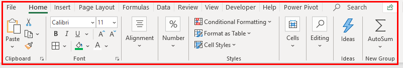
The ribbon is an element of the UI (User Interface) at the top of Excel. In simple words, the ribbon can be called a strip consisting of buttons or tabs seen at the top of the Excel sheet. The ribbon was first introduced in Microsoft Excel in 2007.

In an earlier version of Excel, a menu and toolbar were replaced by a ribbon 2007. The basic tabs under the ribbon are – “Home,” “Insert,” “Page Layout,” “Formulas,” “Data,” “Review,” and “View.” We can customize it according to the requirements. See the image below. The highlighted strip is called ribbon, consisting of tabs like “Home, “Insert,” etc.

How to Customize Ribbon in Excel?

Below are the steps to customize the ribbon.

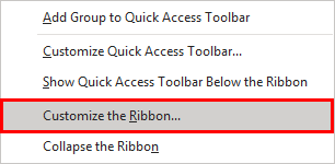
Step 1 – Right-click anywhere on the ribbon. It will open a pop-up with options, including “Customize the Ribbon.”

Step 2 – This will open the Excel Options box for you.

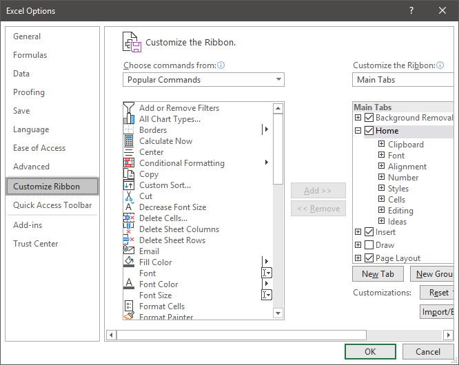
Step 3 – You can see two options on the screen: “Customize the Ribbon” on the right and the “Choose commands from” option on the left.

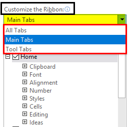
In the dropdown below, there are three options to customize the ribbon. By default, the “Main Tabs” is selected. The other two are “Tool Tabs” and “All Tabs.”

Step 4 – You can click on the (+) sign to expand the list.

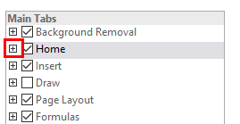
You will see some more tabs under the Main Tabs.

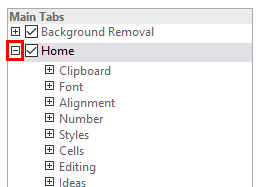
You can shrink the list by clicking on the (-) sign.

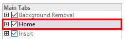
Step 5 – You can select or deselect the required tab to customize the ribbon. It will appear on the sheet accordingly.

You can also add additional tabs to your sheet by following the below steps.

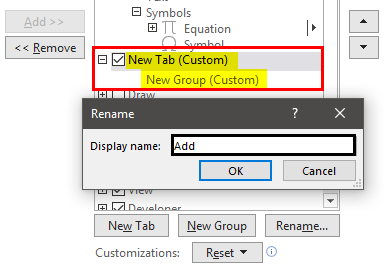
Click New Tab or New group and rename it with some name (not necessary) by clicking on the rename option.
Go to choose a command from option and select the desired option from the dropdown.
Add command to the tab or group you have created.

Click on File Menu —> Options

It will open Excel options for you, where you will see the option to customize the ribbon.

How to Collapse (Minimize) Ribbon in Excel?

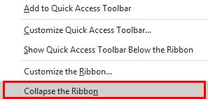
You can collapse the ribbon by right-clicking anywhere on the ribbon and then selecting the “Collapse the Ribbon” option.

How to Use a Ribbon in Excel with Examples

Below are some examples where you required customization of the ribbon.

Example #1

Solution:

We can use excel shortcuts Excel Shortcuts An Excel shortcut is a technique of performing a manual task in a quicker way. read more “Alt + F8” to record macro and “Alt + F11” to open the VBA screen. But remembering shortcuts is not always easy, so here is another option.

Shortcut key to Record Macro:

Shortcut key to Open VBA Screen:

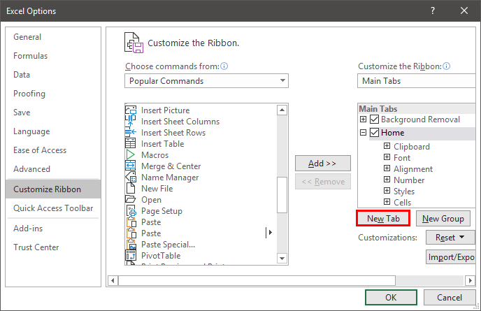
Add developer ribbon in excel by using the following steps. First, “Customize the Ribbon” will open the Excel options box.

Check on the developer option shown in the list under the main tabs. See the image below. Click Ok.

You can see the macros or basic visual screens option.

Example #2

Solution:

The “Power View” option is hidden in Excel 2016. So, we must follow the below steps to add the “Power View” command in our Excel. First, go to “Customize the Ribbon.”

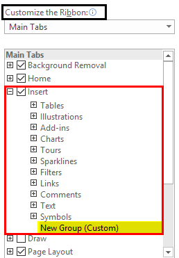
Under “Customize the Ribbon,” extend the “Insert” option, then click on the “New Group (Custom).”

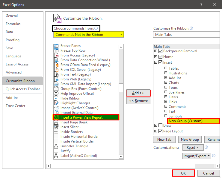
Now, choose the command shown on the left and select the command, not in the ribbon from the dropdown. Now, select “Insert a Power View Report.” Next, click on “Add.” It will add a “Power View” under the “Insert” tab. (When you click on “Add,” make sure a “New Group (Custom)” is selected. Else, an error will pop up). Select “OK.” See the below image:

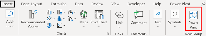
Now you can see the power view option under the insert tab in the new group section:

Example #3

Let’s take another scenario.

Suppose we are working on a report requiring the sum of the values in subsequent rows or columns very frequently.

To sum up the values, we need to write a SUM function whenever the total value is required. Here, we can simplify our work by adding the AutoSum command to our ribbon. Then, go to “Customize the Ribbon.”

Under customize, the ribbon, Extend home, then click on the new group.

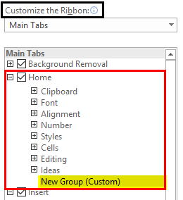
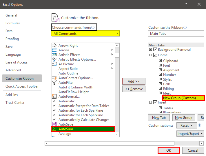
Now, choose the command shown on the left and select “All commands” from the dropdown. Now, select the “∑” AutoSum option. Next, click on “Add.” It will add “∑” “AutoSum” under the “Home” tab. (when you click on “Add,” make sure a “New Group (Custom)” is selected. Else, an error will pop up). Select “OK.” See the below image:

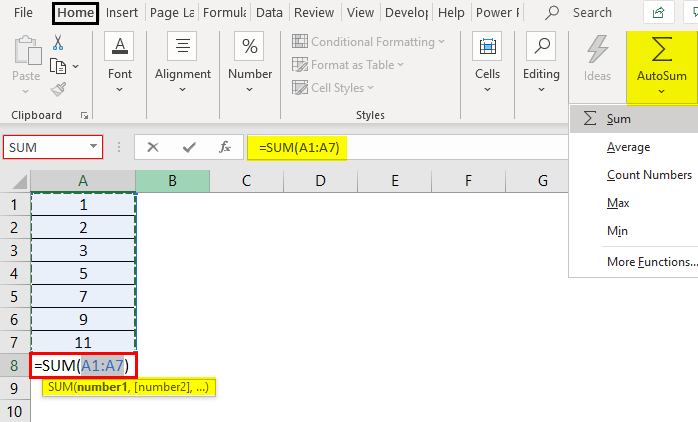
Now you can see the Autosum option under Home Tab in the New Group section:

Now let us see the use of it.

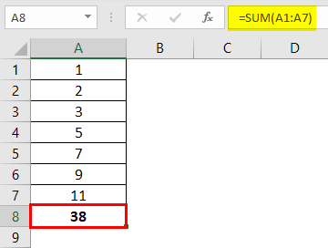
We have some numbers in cells A1 to A7. We need to get the sum in A8. Select cell A8 and click “AutoSum.” It will automatically apply the SUM formula for the active range and give you the SUM.

We get the following result.

Things to Remember

We must slow the performance by adding tabs to the ribbon. So, we must add and keep only those tabs, whichever is required frequently.
We must add a logical command to a logical group or tab so it can easily find that command.
When adding commands from the “Command” option, not the ribbon, we must ensure that we have created a “New Group (Custom).” Otherwise, it will display the error.

Excel VSTO Add-in: Add Ribbon Button and Update Cell Value

by Igor Katenov, the lead developer at 10Tec

Our previous article related to VSTO provides a basic sample demonstrating how to display a form every time when Excel starts. This is not much useful in the real life. Let’s do something more practical now. We customize the Excel interface by adding a Ribbon button to display a dialog in which the user can make a choice and update cell value accordingly:

The dialog will display a list of countries with cultures inside them to select the first day of week in a particular culture. As earlier, we will build an Excel VSTO add-in with VB.NET and Visual Studio.

Step 1: Add a button to the Office Ribbon

Let’s begin. Launch Visual Studio and create a new solution based on the ‘Excel VSTO Add-in’ template. If you cannot find this template in the list of available templates, most likely, your copy of Visual Studio is not configured for Office development with VSTO. In this case, we refer you to the previous article: you will find preliminary instructions for configuring Visual Studio for development with VSTO in it.

Enter any suitable name of the new solution in the ‘Configure your new project’ dialog and hit the Create button:

A new Excel VSTO Add-in solution appears. Our main goal is adding a clickable button to the Office Ribbon. You can add custom items to the Ribbon using a designer like the traditional Windows Forms designer, do this from code or customize the Ribbon in advanced ways with XML. All these techniques are described in the Microsoft documentation — a good starting point is the Ribbon Overview topic in the Office UI Customization section. We will create a Ribbon button the simplest way, i.e. visually with the Ribbon Designer.

Select the ‘Add New Item…’ command from the Project menu of Visual Studio or from the context menu of our Excel VSTO Add-in project. In the ‘Add New Item’ dialog, select the ‘Ribbon (Visual Designer)’ item and click the Add button:

The Ribbon Designer opens, displaying the default Add-ins tab and one Ribbon group inside it. To add a button to the Ribbon, drag the Button control from the ‘Office Ribbon Controls’ group in the Visual Studio Toolbox to the only group named Group1:

Hit F5 to test our VSTO add-in. Excel opens, and we should see the created Button1 on the Add-ins tab in the Office Ribbon when we switch to this tab:

If you do not see the Add-ins tab, it may be hidden by default. To enable it, open the ‘Customize Ribbon’ tab in the Excel options dialog and tick the Add-ins item in the list of available Ribbon tabs:

Well, the first task is done – we have just added a button to the Ribbon. If you want, you can change the button caption to something more understandable like ‘Select Country’. Select the added Button1 control and change its Text property in the Visual Studio property grid accordingly.

Step 2: Create a dialog with country list

We already have a Ribbon button, and we want to show a dialog when the user clicks it. Now is the right time to create a Windows Forms form that will be used as the dialog and populate it. We will use our WinForms grid control named iGrid.NET to show the country list to select from.

First we add a new empty form to our Excel VSTO add-in solution by choosing the ‘Add Form (Windows Forms)…’ command from the Project menu or from the project’s context menu in the Solution Explorer. Then drag the iGrid icon from the Visual Studio Toolbox to the form to create an instance of the iGrid control that will display a country list. Position the grid control on the form and change the form title to have something like this:

The grid will be populated with countries and cultures available inside every country in the form’s Load event handler. Double-click the form’s title to create a stub for the Form1_Load method. First add some Imports directives for the used types at the top of the module — they will help us to make our code a little bit cleaner:

Now make the form’s Load event handler looking like the following code snippet:

We create 3 columns in iGrid, populate it with data, and set some visual and behavior settings. Our grid will look like a multi-column list box with vertical grid lines between columns; it will be sorted by the Country column, and the user will be able to find the required country by typing its first characters like on the screenshot at the top of this article.

Step 3: Show the dialog and update cell value

The dialog with country list should appear on the screen when the user clicks the ‘Select Country’ button on the Ribbon. Let’s write the corresponding event handler for this Ribbon button. Switch to the ‘Ribbon1.vb [Design]’ tab in the Visual Studio workspace and double-click the Ribbon button we added earlier. A stub for the button’s Click event handler appears in the code module of the Ribbon. Create an instance of the Form1 class and call its ShowDialog() method in this event handler:

If you are eager to see the result of our work, hit F5 in Visual Studio to launch the new version of our Excel VSTO add-in. After Excel popped up, open the Add-ins tab in the Ribbon and click the ‘Select Country’ button in it. The dialog populated with the data we expect to see must appear:

The only remaining part of work is updating of the value of the active cell when the user hits ENTER on the selected item. This work will be done in the KeyDown event handler of iGrid. Return to the form’s code module (Form1.vb) and put the following event handler in it:

That’s all. You can hit F5 again, select a country in the list and click ENTER to make sure that the First Day of Week value from the selected item is placed into the active worksheet cell.

Wrapping up

An Excel VSTO add-in solution built in this article shows how to add a Ribbon button and display a dialog to update the value of the active worksheet cell. We were developing this add-in with Visual Studio that automatically registers our add-in in Excel. This means our add-in will load and become available in every copy of Excel. If you do not need this, don’t forget to clean your solution with the BuildClean Solution command in Visual Studio. This command also unregisters the add-in if you work with VSTO add-in solutions.

Источник

Заметим также, что эта сборка успешно работает и с новыми версиями Excel, включая 2010 и 2013. Сборки более ранних версий не имеют возможности для создания Ribbon интерфейсов.
Ключевым элементов этой сборки является интерфейс IRibbonExtensibility, который собственно и позволяет создавать Ribbon элементы.

[ComVisible(true)]

public class ComAddin : IDTExtensibility2, IRibbonExtensibility

{

public string GetCustomUI(string ribbonID)

{

throw new NotImplementedException();

}

…

}

Единственным методом является GetCustomUI который возвращает строку, содержащую описание Ribbon интерфейса в виде XML. Excel, в свою очередь, при загрузке надстройки обновит Ribbon интерфейс на основе этого описания.
Visual Studio не располагает дизайнером для создания Ribbon интерфейсов (если речь не идет о VSTO), поэтому создадим описание элементов интерфейса вручную. Для этого добавим к проекту XML файл.

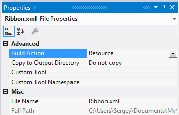
Для вновь созданного файла установим свойство Build Action в значение Resource.

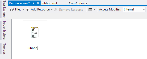
После чего добавим к проекту файл ресурсов.

Откроем вновь созданные файл ресурсов и перетащим в открывшееся окно наш XML файл.

После всех этих манипуляций мы можем обратиться к XML файлу, расположенному в ресурсах и получить его содержимое в виде строки. Обновим метод GetCusomUI следующим образом.

public string GetCustomUI(string ribbonID)

{

return Resources.Ribbon;

}

Таким образом, метод возвращает строку, представляющую собой пользовательский интерфейс в виде XML. Осталось самое главное — описать элементы интерфейса.

<?xml version=«1.0« encoding=«UTF-8«?>

<tabs>

</box>

</menu>

</group>

</tab>

</tabs>

</ribbon>

Разберемся подробнее. Корневым элементом является customUI, в качестве атрибута xmlns принимающий значение «http://schemas.microsoft.com/office/2006/01/customui». Namespace указывает на причастность к Excel 2007. Как уже писалось выше, этот интерфейс будет работать и в более свежих версиях Excel. Однако для доступа к новым функциям, таким как активация Ribbon вкладки при запуске Excel или авто-масштабирование, появившимся в Excel 2010, необходимо использовать namespace «http://schemas.microsoft.com/office/2009/07/customui» и, соответственно, сборку office.dll с номером версии 14.
Элемент tab представляет новую вкладку с именем «First COM Add-in». Заметим, что идентификатор id является обязательным для всех элементов интерфейса. В случае отсутствия идентификатора у элемента, сам элемент отображен не будет. При этом никакого сообщения об ошибки не выведется.
Каждая вкладка может содержать несколько групп элементов. Группы, в свою очередь, содержат сами элементы управления. В нашем случае мы добавили одну группу с именем «Ribbon».

<group id=«myGroup« label=«Ribbon«>
…

</group>
</tab>

Элемент button, как понятно из названия, представляет собой кнопку. Атрибут size задает размер кнопки («large» или «normal»). Атрибут label задает текст кнопки. Для установки изображения кнопки, в данном случае используется атрибут imageMso, которые указывает на одну из встроенных иконок. Для задания собственной иконки используется атрибуты image или getImage.

Элемент box представляет собой группу элементов, расположенных вертикально или горизонтально. Способ расположения элементов указывается с помощь атрибута boxStyle. Элемент toggleButton представляет собой западающую кнопку, в то время как checkbox — это обычный флажок.

Элемент menu представляет собой кнопку с выпадающим меню. В данном случае меню состоит из 3-х элементов.

</menu>

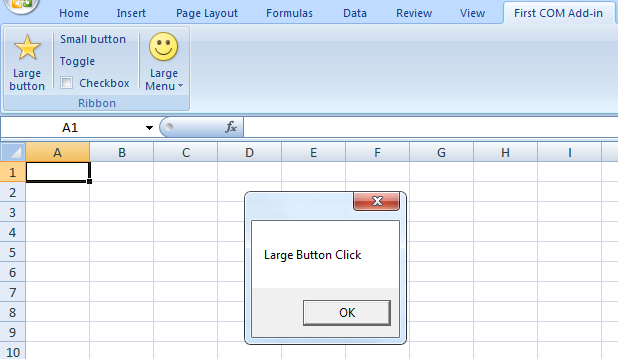
После регистрации обновленной надстройки, Excel добавит новую вкладку на панель.

Callback методы

Ribbon добавлен, однако обработка событий элементов управления не происходит. Для этого необходимо описать callback методы, т.е. методы класса, которые будут вызваны при возникновении того или иного события.

<?xml version=«1.0« encoding=«UTF-8«?>

<tabs>

</box>

</menu>

</group>

</tab>

</tabs>

</ribbon>

</customUI>

Для описания callback методов используются атрибуты начинающиеся, как правило, со слова «on» или «get». При этом атрибут задает имя метода, который будет вызван при возникновении события. Требования к callback методам следующие:

Идентификатор доступа должен быть public;
Имя метода должно совпадать со значением, установленном в соответствующем атрибуте, включая регистр;
Сигнатура метода должна соответствовать типу события.

Одно и то же событие имеет разную сигнатуру callback методов. Так, событие onAction для элемента button требует следующую сигнатуру callback метода

void OnAction(IRibbonControl control)

Для элементов checkbox и togglebutton, сигнатура метода должна быть

void OnAction(IRibbonControl control, bool pressed)

Список всех callback методов и их сигнатур доступен по ссылке.

Почти все callback методы получают объект типа IRibbonControl, которые содержит информацию об элементе, инициировавшем событие. Свойства Id, например, возвращает идентификатор элемента. Это свойство полезно, в случае, если несколько элементов используют один callback метод, таким образом можно определить какой именно элемент сгенерировал событие.

Добавим реализацию callback методов.

public string OnGetLabel(IRibbonControl control)

{

switch (control.Id)

{

case «buttonLarge»:

return «Large button»;

default:

return null;

}

public void OnLargeButtonClick(IRibbonControl
control)

{

MessageBox.Show(«Large Button Click»);

}

public void OnSmallButtonClick(IRibbonControl
control)

{

MessageBox.Show(«Small Button Click»);

}

public void OnCheckBoxClick(IRibbonControl
control, bool pressed)

{

MessageBox.Show(«Checkbox Click: « + (pressed ? «checked» : «unchecked»));

}

public void OnToggleClick(IRibbonControl
control, bool pressed)

{

MessageBox.Show(«Toggle Button Click: « + (pressed ? «checked» : «unchecked»));

}

public void OnMenuButtonClick(IRibbonControl
control)

{

MessageBox.Show(«Menu Button Click: « + control.Id);

Событие getLabel (callback метод OnGetLabel) срабатывает при перерисовки Ribbon интерфейса и возвращает текст для соответствующего элемента. В нашем случае мы проверяем элемент управления, инициировавший событие, и возвращаем текст для этого элемента. Этот метод полезен если необходимо добавить поддержку нескольких языков и отображать разный текст на разных языках.

public string OnGetLabel(IRibbonControl control)

{

switch (control.Id)

{

case «buttonLarge»:

return «Large button»;

default:

return null;

}

Событие onAction для кнопки срабатывает при её нажатии. В качестве единственного аргумента callback метод получает объект типа IRibbonControl.

public void OnLargeButtonClick(IRibbonControl control)

{

MessageBox.Show(«Large Button Click»);

}

Для элементов togglebutton и checkbox, callback метод также содержит переменную типа bool, которая указывает, какое состояние принял элемент.

public void OnCheckBoxClick(IRibbonControl control, bool pressed)

{

MessageBox.Show(«Checkbox Click: « + (pressed ? «checked» : «unchecked»));

}

Соберем проект и зарегистрируем обновленную сборку. При тестировании в Excel видим обработку событий для элементов управления.

С исходниками проекта и готовой надстройкой можно ознакомиться по ссылке.

Источник

Why use Excel Add-in

Save Excel Add-In

Install Excel Add-in (User)

Remove Excel Add-in

JUST LAUNCHED!

Step 1: Download The Template

Step 2: Link Your Macros

1. Hide Unused Groups & Buttons

2. Add Your Macro Code

3. Add A Screentip For Your Macros

4. Add Your Tab, Group, & Button Names To The Ribbon UI

Step 3: Test Your Buttons

Step 4: Choose Your Icons

How Do You Get The Icon Names?

How Do You Change The Icon Size?

Step 5: Save File As An Add-in

Congratulations, You Have Developed Your First Add-in!

Want More Features? Check Out My First Add-in

About The Author

Ribbon in Excel

What is Ribbon in Excel?

Table of contents

How to Customize Ribbon in Excel?

How to Collapse (Minimize) Ribbon in Excel?

How to Use a Ribbon in Excel with Examples

Example #1

Example #2

Example #3

Things to Remember

Recommended Articles

Excel VSTO Add-in: Add Ribbon Button and Update Cell Value

Step 1: Add a button to the Office Ribbon

Step 2: Create a dialog with country list

Step 3: Show the dialog and update cell value

Wrapping up

Callback методы