Excel return value from array

I can’t see a short and snappy answer to this but here is one suggestion assuming the data starts in column A

=INDEX(2:2,AGGREGATE(15,6,COLUMN(INDEX(2:2,MATCH(1,2:2,0)):INDEX(2:2,MATCH(999,2:2)))/(INDEX(2:2,MATCH(1,2:2,0)):INDEX(2:2,MATCH(999,2:2))>1),1))

If the range didn’t start in column A, you would have to subtract the number of the column before the first column of the range from the column number returned by the AGGREGATE to get the correct index value relative to the start of the array e.g. for B2:Z2

=INDEX(B2:Z2,AGGREGATE(15,6,COLUMN(INDEX(B2:Z2,MATCH(1,B2:Z2,0)):INDEX(B2:Z2,MATCH(999,B2:Z2)))/(INDEX(B2:Z2,MATCH(1,B2:Z2,0)):INDEX(B2:Z2,MATCH(999,B2:Z2))>1),1)-COLUMN(A:A))

To be honest it wouldn’t be worth using a MATCH to find the last number in the range unless the number of cells in the range was very large, so the formula for B2:Z2 would just be

=INDEX(B2:Z2,AGGREGATE(15,6,COLUMN(INDEX(B2:Z2,MATCH(1,B2:Z2,0)):Z2)/(INDEX(B2:Z2,MATCH(1,B2:Z2,0)):Z2>1),1)-COLUMN(A:A))

Formula starting column A

Formula starting at column B

Key Points

• Think of an array in VBA array as a mini database to store and organized data (Example: student’s name, subject, and scores).
• Before you use it, you need to declare an array; with its data type, and the number of values you want to store in it.

If you want to work with large data using VBA, then you need to understand arrays and how to use them in VBA codes, and in this guide, you will be exploring all the aspects of the array and we will also see some examples to use them.

What is an Array in VBA?

In VBA, an array is a variable that can store multiple values. You can access all the values from that array at once or you can also access a single value by specifying its index number which is the position of that value in the array. Imagine you have a date with student’s name, subject, and scores.

You can store all this information in an array, not just for one student but for hundreds. Here’s a simple example to explain an array.

In the above example, you have an array with ten elements (size of the array) and each element has a specific position (Index).

So, if you want to use an element that is in the eighth position you need to refer to that element using its index number.

The array that we have used in the above example is a single-dimension array. But ahead in this guide, we will learn about multidimensional arrays as well.

How to Declare an Array in VBA

As I mentioned above an array is the kind of variable, so you need to declare it using the keywords (Dim, Private, Public, and Static). Unlike a normal variable, when you declare an array you need to use a pair of parentheses after the array’s name.

Let’s say you want to declare an array that we have used in the above example.

Steps to declare an array.

Full Code

Sub vba_array_example()
Dim StudentsNames(10) As String
StudentsNames(0) = "Waylon"
StudentsNames(1) = "Morton"
StudentsNames(2) = "Rudolph"
StudentsNames(3) = "Georgene"
StudentsNames(4) = "Billi"
StudentsNames(5) = "Enid"
StudentsNames(6) = "Genevieve"
StudentsNames(7) = "Judi"
StudentsNames(8) = "Madaline"
StudentsNames(9) = "Elton"
End Sub

Quick Notes

• In the above code, first, you have the Dim statement that defines the one-dimensional array which can store up to 10 elements and has a string data type.
• After that, you have 10 lines of code that define the elements of an array from 0 to 9.

Array with a Variant Data Type

While declaring an array if you omit to specify the data type VBA will automatically use the variant data type, which causes slightly increased memory usage, and this increase in memory usage could slow the performance of the code.

So, it’s better to define a specific data type when you are declaring an array unless there is a need to use the variant data type.

Returning Information from an Array

As I mentioned earlier to get information from an array you can use the index number of the element to specify its position. For example, if you want to return the 8th item in the area that we have created in the earlier example, the code would be:

In the above code, you have entered the value in cell A1 by using item 8 from the array.

Use Option Base 1

I’m sure you have this question in your mind right now why we’re started our list of elements from zero instead of one?

Well, this is not a mistake.

When programming languages were first constructed some carelessness made this structure for listing elements in an array. In most programming languages, you can find the same structure of listing elements.

However, unlike most other computer languages, In VBA you can normalize the way the is index work which means you can make it begins with 1. The only thing you need to do is add an option-based statement at the start of the module before declaring an array.

Now this array will look something like the below:

Searching through an Array

When you store values in an array there could be a time when you need to search within an array.

In that case, you need to know the methods that you can use. Now, look at the below code that can help you to understand how to search for a value in an array.

Sub vba_array_search()

'this section declares an array and variables _
that you need to search within the array.
Dim myArray(10) As Integer
Dim i As Integer
Dim varUserNumber As Variant
Dim strMsg As String

'This part of the code adds 10 random numbers to _
the array and shows the result in the _
immediate window as well.
For i = 1 To 10
myArray(i) = Int(Rnd * 10)
Debug.Print myArray(i)
Next i

'it is an input box that asks you the number that you want to find.
Loopback:
varUserNumber = InputBox _
("Enter a number between 1 and 10 to search for:", _
"Linear Search Demonstrator")

'it's an IF statement that checks for the value that you _
have entered in the input box.
If varUserNumber = "" Then End
If Not IsNumeric(varUserNumber) Then GoTo Loopback
If varUserNumber < 1 Or varUserNumber > 10 Then GoTo Loopback

'message to show if the value doesn't found.
strMsg = "Your value, " & varUserNumber & _
", was not found in the array."

'loop through the array and match each value with the _
the value you have entered in the input box.
For i = 1 To UBound(myArray)
If myArray(i) = varUserNumber Then
strMsg = "Your value, " & varUserNumber & _
", was found at position " & i & " in the array."
Exit For
End If
Next i

'message box in the end
MsgBox strMsg, vbOKOnly + vbInformation, "Linear Search Result"

End Sub

1. In the first part of the code, you have variables that you need to use in the code further.
2. After that, the next part is to generate random numbers by using RND to get you 10 values for the array.
3. Next, an input box to let enter the value that you want to search within the array.
4. In this part, you have a code for the string to use in the message box if the value you have entered is not found.
5. This part of the code uses a loop to loop through each item in the array and check if the value that you have entered is in the array or not.
6. The last part of the code shows you a message about whether a value is found or not.

Author: Oscar Cronquist Article last updated on February 22, 2023

The VLOOKUP function is designed to return only a corresponding value of the first instance of a lookup value, from a column you choose. But there is a workaround to identify multiple matches.

The array formulas demonstrated below are smaller and easier to understand and troubleshoot than the useful VLOOKUP function.

However you are not limited to array formulas, Excel also has built-in features that work very well, you will be amazed at how easy it is to filter values in a data set.

I have made a formula, demonstrated in a separate article, that allows you to VLOOKUP and return multiple values across worksheets, there is also an Add-In that makes it even easier to accomplish this task.

Now, if you only need one instance of each returned value then check this article out: Vlookup – Return multiple unique distinct values It lets you specify a condition and the formula is not even an array formula.

I have also written an article about searching for a string (wildcard search) and return corresponding values, it requires a somewhat more complicated formula but don’t worry, you will find an explanation there, as well.

Did you know that it is also possible to VLOOKUP and return multiple values distributed over several columns, the formula even ignores blanks.

1. VLOOKUP — Return multiple values vertically

Can VLOOKUP return multiple values? It can, however the formula would become huge if it needs to contain the VLOOKUP function. The formula presented here does not contain that function, however, it is more versatile and smaller.

The image above shows you an array formula that extracts adjacent values based on a lookup value in cell D10.

Another great thing with this array formula is that it allows you to lookup and return values from whatever column you like contrary to the VLOOKUP function that lets you only do a lookup in the left-most column, in a given range.

Update 17 December 2020, check out the new FILTER function available for Excel 365 users. Regular formula in cell D10:

=FILTER(C3:C7, B10=B3:B$7)

Read here about how it works: Filter values based on a condition

The following formula is for earlier Excel versions. Array formula in D10:

=INDEX($C$3:$C$7, SMALL(IF(($B$10=$B$3:$B$7), MATCH(ROW($B$3:$B$7), ROW($B$3:$B$7)), «»),ROWS($A$1:A1)))

This video explains how to VLOOKUP and return multiple matching values:

The array formula in cell G3 looks in column B for «France» and return adjacent values from column C. The array formula in cell G3 filters values unsorted, if you want to sort returning values alphabetically, read this:
Vlookup with 2 or more lookup criteria and return multiple matches

How to create an array formula

1. Copy array formula above. (Ctrl + c)
2. Double-press with left mouse button on a cell.
3. Paste (Ctrl + v) array formula.
4. Press and hold Ctrl + Shift simultaneously.
5. Press Enter once.
6. Release all keys.

Read more

How to enter an array formula | Convert array formula to a regular formula | How to enter array formulas in merged cells

Back to top

The array formula above filters only values with one condition, the following article explains how to filter based on multiple criteria: Vlookup with 2 or more lookup criteria and return multiple matches

If you don’t like array formulas, try this regular but more complicated formula in cell D10:

=INDEX($C$3:$C$7,SMALL(INDEX(($B$10=$B$3:$B$7)*(MATCH(ROW($B$3:$B$7), ROW($B$3:$B$7)))+($E$3<>$B$3:$B$7)*1048577,),ROWS($A$1:A1)))

Back to top

Explaining array formula (Return values vertically)

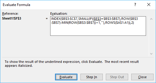
You can easily follow along as I explain the formula, select cell D10. Go to tab «Formulas» on the ribbon and press with left mouse button on «Evaluate Formula» button. Press with left mouse button on «Evaluate» button shown above to move to next step.

Step 1 — Identify cells equal to the condition in cell B10

= (equal sign) is a comparison operator and checks if criterion (E3) is equal to values in array ($B$3:$B$7). This operator is not case sensitive.

$B$10=$B$3:$B$7

becomes

«France«={«Germany»;»Italy»;»France«;»Italy»;»France«}

and returns

{FALSE, FALSE, TRUE, FALSE, TRUE}

The image above shows an array in cell range D3:D7 containing boolean values, those values correspond to the logical expression if cell B10 is equal B3:B7. Cell B5 and B7 is equal to cell B10, these return TRUE. The other remaining cells is not equal to cell B10 and return FALSE.

Step 2 — Create array containing corresponding row numbers

The ROW function returns the row number based on a cell reference, we are using a cell reference that points to a cell range containing multiple rows so the ROW function returns an array of row numbers.

MATCH(ROW($B$3:$B$7), ROW($B$3:$B$7))

The MATCH function finds the relative position of a value in a cell range or array, however, I am using multiple values so this step returns an array of numbers.

MATCH(ROW($B$3:$B$7), ROW($B$3:$B$7))

becomes

MATCH({3, 4, 5, 6, 7}, {3, 4, 5, 6, 7})

and returns {1,2,3,4,5}

The image above shows the array in cell range D3:D7, the array always begins with 1 and has must have the same number of values in the array as the table has rows.

Step 3 — Filter row numbers equal to a condition

The IF function has three arguments, the first one must be a logical expression. If the expression evaluates to TRUE then one thing happens (argument 2) and if FALSE another thing happens (argument 3).

IF(($B$10=$B$3:$B$7), MATCH(ROW($B$3:$B$7), ROW($B$3:$B$7)), «»)

becomes

IF(FALSE, FALSE, TRUE, FALSE, TRUE}, MATCH(ROW($B$3:$B$7), ROW($B$3:$B$7)), «»)

becomes

IF(FALSE, FALSE, TRUE, FALSE, TRUE},{1, 2, 3, 4, 5}, «»)

and returns {«», «», 3, «», 5}

The IF function replaces the numbers that correspond to boolean value FALSE with «» (nothing) and boolean value TRUE with a number, shown in cell range D3:D7.

Step 4 — Return the k-th smallest row number

To be able to return a new value in a cell each I use the SMALL function to filter row numbers from smallest to largest.

The ROWS function keeps track of the numbers based on an expanding cell reference. It will expand as the formula is copied to the cells below.

SMALL(IF(($E$3=$B$3:$B$7),ROW($B$3:$B$7)-MIN(ROW($B$3:$B$7))+1,»»),ROWS($A$1:A1))

becomes

SMALL({«», «», 3, «», 5}, ROWS($A$1:A1))

This part of the formula returns the k-th smallest number in the array {«», «», 3, «», 5}

To calcualte the k-th smallest value I am using ROWS($A$1:A1) to create the number 1.

When the formula in cell D10 is copied to cell D11, ROWS($A$1:A1) changes to ROWS($A$1:A2). ROWS($A$1:A2) returns 2.

In Cell D10: =INDEX($C$3:$C$7, SMALL({«», «», 3, «», 5}, ROWS($A$1:A1))

=INDEX($C$3:$C$7, SMALL({«», «», 3, «», 5}, 1))

The smallest number in array {«», «», 3, «», 5} is 3.

In Cell D11: =INDEX($C$3:$C$7, SMALL({«», «», 3, «», 5}, ROWS($A$1:A2)))

=INDEX($C$3:$C$7, SMALL({«», «», 3, «», 5}, 2))

The second smallest number in array {«», «», 3, «», 5} is 5.

Step 4 — Return value based on row number

The INDEX function returns a value based on a cell reference and column/row numbers.

In Cell D10:

=INDEX($C$3:$C$7, 3)

becomes

=INDEX({«Pear», «Orange», «Apple», «Banana», «Lemon»}, 3)

and returns «Apple» in cell D10.

In Cell D11:

=INDEX($C$3:$C$7, 5) returns «Lemon»

This article demonstrates how to filter an Excel defined table programmatically based on a condition using event code and a macro.

Back to top

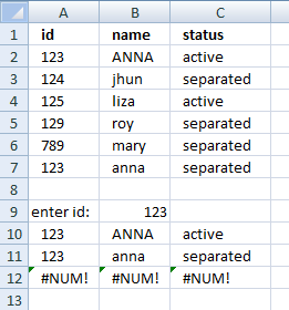
1.1 Return multiple values — case sensitive

The image above demonstrates a formula in cell C10 that extracts values from cell range C3:C7 if the corresponding value in cell range B3:B7 is equal to the value in cell B10.

The values in cell B3:B7  must have the same upper and lower letters as the lookup value in cell B10 to generate a match.

Lookup value «france» is found in cell B3 and B7 but not in cell B5. Cell B5 has a value that begins with an upper letter. The corresponding cells to B3 and B7 are C3 and C7, those values are returned in cell C10 and cells below.

Array formula in cell C10:

=INDEX($C$3:$C$7, SMALL(IF(EXACT($B$10, $B$3:$B$7), MATCH(ROW($B$3:$B$7), ROW($B$3:$B$7)), «»), ROWS($A$1:A1)))

How to enter an array formula

Copy cell C10 and paste to cells below.

If you own Excel 365 you can use the much easier FILTER function to accomplish the same thing: Filter values based on a condition — case sensitive

Back to top

1.2 Return multiple values — if not equal to

The picture above shows an array formula in cell C10 that extracts values from cell range C3:C7 if the corresponding value in cell range B3:B7 is NOT equal to the lookup value in cell B10.

The lookup value in cell B10 is not equal to the value in B3, B4, and B6. The corresponding values in C3, C4, and C6 are returned to cell C10 and cells below.

Array formula in cell C10:

=INDEX($C$3:$C$7, SMALL(IF($B$10<>$B$3:$B$7, MATCH(ROW($B$3:$B$7), ROW($B$3:$B$7)), «»), ROWS($A$1:A1)))

How to enter an array formula

Copy cell C10 and paste to cells below.

If you own Excel 365 you can use the much easier FILTER function to accomplish the same thing: Filter values if not equal to

Back to top

1.3 Return multiple values — if smaller than

The image above demonstrates a formula in cell C10 that extracts items from cell range B3:B7 if the corresponding value in cell range C3:C7 is smaller than the value in cell B10.

In the example above, cells C5 and C7 are smaller than the value in cell B10. The corresponding cells are B5 and B7 which the formula returns in cell C10 and cells below.

Array formula in cell C10:

=INDEX($B$3:$B$7, SMALL(IF($B$10>$C$3:$C$7, MATCH(ROW($B$3:$B$7), ROW($B$3:$B$7)), «»), ROWS($A$1:A1)))

How to enter an array formula

Copy cell C10 and paste to cells below.

If you own Excel 365 you can use the much easier FILTER function to accomplish the same thing: Filter values if smaller than

Back to top

1.4 Return multiple values — if larger than

The picture above demonstrates a formula in cell C10 that extracts values from cell range B3:B7 if the corresponding values in C3:C7 are less than the value in cell B10.

In this example, cells C5 and C7 are smaller than the value in cell B10. The formula in cell C10 returns the corresponding values from B5 and B7.

Array formula in cell C10:

=INDEX($B$3:$B$7, SMALL(IF($B$10<$C$3:$C$7, MATCH(ROW($B$3:$B$7), ROW($B$3:$B$7)), «»), ROWS($A$1:A1)))

How to enter an array formula

Copy cell C10 and paste to cells below.

If you own Excel 365 you can use the much easier FILTER function to accomplish the same thing: Filter values if smaller than

Back to top

1.5 Return multiple values — if contains

The image above demonstrates a formula in cell C10 that extracts values from cell range C3:C7 if the corresponding values in cell range B3:B7 contain the value in cell B10.

In this example, the values in cells B3, B5, and B7 contain the value in cell B10. The array formula returns the corresponding values from cells C3, C5, and C7 to cell C10 and cells below as far as necessary.

Array formula in cell C10:

=INDEX($C$3:$C$7, SMALL(IF(ISNUMBER(SEARCH($B$10, $B$3:$B$7)), MATCH(ROW($B$3:$B$7), ROW($B$3:$B$7)), «»), ROWS($A$1:A1)))

How to enter an array formula

Copy cell C10 and paste to cells below.

If you own Excel 365 you can use the much easier FILTER function to accomplish the same thing: Filter values if contains

Back to top

1.6 Return multiple values — if not contains

The picture above demonstrates a formula in cell C10 that extracts values from cell range C3:C7 if the corresponding values in cell range B3:B7 do not contain the value in cell B10.

In this example, the values in cells B4, and B6 do not contain the value in cell B10. The array formula returns the corresponding values from cells C4, and C6 to cell C10 and cells below as far as necessary.

Array formula in cell C10:

=INDEX($C$3:$C$7, SMALL(IF(ISNUMBER(SEARCH($B$10, $B$3:$B$7)), «», MATCH(ROW($B$3:$B$7), ROW($B$3:$B$7))), ROWS($A$1:A1)))

How to enter an array formula

Copy cell C10 and paste to cells below.

If you own Excel 365 you can use the much easier FILTER function to accomplish the same thing: Filter values if contains

Back to top

1.7 Return multiple values — that begins with

The formula in cell C10 extracts values from cell range C3:C7 if the corresponding values in B3:B7 begin with the same value as the value entered in cell B10.

The image above shows that cell B4 and B6 begins with the same value as the value in cell B10. The corresponding values in cell C4 and C6 are displayed in cell C10 and C11.

Array formula in cell C10:

=INDEX($C$3:$C$7, SMALL(IF($B$10=LEFT($B$3:$B$7, LEN($B$10)), MATCH(ROW($B$3:$B$7), ROW($B$3:$B$7)), «»), ROWS($A$1:A1)))

How to enter an array formula

Copy cell C10 and paste to cells below as far as needed.

If you own Excel 365 you can use the much easier FILTER function to accomplish the same thing: Filter values that begin with

Back to top

1.8 Return multiple values — that ends with

Array formula in cell C10:

=INDEX($C$3:$C$7, SMALL(IF(RIGHT($B$3:$B$7, LEN($B$10))=$B$10, MATCH(ROW($B$3:$B$7), ROW($B$3:$B$7)), «»), ROWS($A$1:A1)))

How to enter an array formula

Copy cell C10 and paste to cells below as far as needed.

If you own Excel 365 you can use the much easier FILTER function to accomplish the same thing: Filter values that end with

Back to top

How to remove #num errors

The picture above shows you the array formula copied down to cell D12 however there are only two values shown, the remaining cells show nothing not even an error.

Array formula in cell D10:

=IFERROR(INDEX($C$3:$C$7, SMALL(IF(($B$10=$B$3:$B$7), MATCH(ROW($B$3:$B$7), ROW($B$3:$B$7)), «»),ROWS($A$1:A1))), «»)

The IFERROR function lets you convert error values to blank cells or really in whatever value you want. In this case it returns blank cells.

Note: The IFERROR catches all kinds of formula errors. you won’t spot the error that easily if there is some kind of other error in the formula. Use this function with caution.

How to enter an array formula

Recommended articles

How to use the IFERROR function  | How to use the ISERROR function | How to use the ERROR.TYPE function | How to find errors in a worksheet | Delete blanks and errors in a list

Back to top

1.9 Count matching values

The following image shows you a data set in column B and C. The lookup value in cell E3 is used for identifying matching cell values in column B.

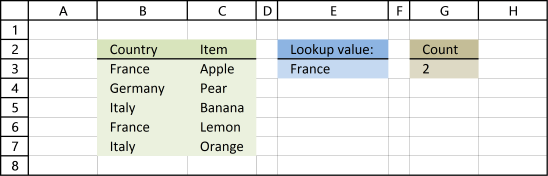
Formula in cell G3:

=COUNTIF($B$3:$B$7,E3)

Alternative formula in cell G3:

=SUMPRODUCT(($B$3:$B$7=E3)*1)

Recommended articles

Count a given pattern in a cell value | Count cells containing text from list | Count cells between specified values | Count entries based on date and time | Count unique distinct values | Count unique distinct records |

Back to top

2. Return multiple values horizontally

Update 17 December 2020, use the FILTER function to return multiple values horizontally. Regular formula in cell C10:

=TRANSPOSE(FILTER(C3:C7, B10=B3:B7))

The formula above works only in Excel 365. The array formula below is for earlier Excel versions and is entered in cell C10.

Array formula in C10:

=INDEX($C$3:$C$7, SMALL(IF($B$10=$B$3:$B$7, ROW($B$3:$B$7)-MIN(ROW($B$3:$B$7))+1, «»), COLUMNS($A$1:A1)))

Copy cell C10 and paste to cells to the right of cell C10 as far as needed.

Enter the formula above  as an array formula or use this regular but more complicated formula:

=INDEX($C$3:$C$7, SMALL(INDEX(($B$10=$B$3:$B$7)*(MATCH(ROW($B$3:$B$7), ROW($B$3:$B$7))+($B$19<>$B$3:$B$7)*1048577, 0, 0), COLUMNS($A$1:A1)))

Back to top

Recommended articles

Search values distributed horizontally and return corresponding values | Resize a range of values | Rearrange values | Rearrange cells in a cell range to vertically distributed values | Rearrange values based on category(VBA) | Normalize data (VBA) | Normalize data, part 2 |

3. Extract multiple records based on a condition

Update 17 December 2020, use the new FILTER function to extract values based on a condition, formula in cell A10:

=FILTER(A2:C7, B9=A2:A7)

The FILTER function is available for Excel 365 users and the formula above is entered as a regular formula.

The formula below is for earlier Excel versions, it extracts records based on the value in cell B9. Array formula in cell A10:

=INDEX($A$2:$C$7, SMALL(IF($B$9=$A$2:$A$7, ROW($A$2:$A$7)-MIN(ROW($A$2:$A$7))+1, «»), ROW(A1)),COLUMN(A1))

To enter an array formula, type the formula in a cell then press and hold CTRL + SHIFT simultaneously, now press Enter once. Release all keys.

The formula bar now shows the formula with a beginning and ending curly bracket telling you that you entered the formula successfully. Don’t enter the curly brackets yourself.

Copy cell A10 and paste to cell range B10:C10. Then copy A10:C10 and paste to cell range A11:C12.

3.1 Watch a video where I explain how to use the array formula and how it works

Enter the formula above as an array formula or use this regular but more complicated formula:

=INDEX($A$2:$C$7, SMALL(INDEX(($B$9=$A$2:$A$7)*(MATCH(ROW($A$2:$A$7), ROW($A$2:$A$7)))+($B$9<>$A$2:$A$7)*1048577, 0, 0),ROW(A1)),COLUMN(A1))

Recommended reading

• Extract all rows from a range that meet criteria in one column
• Match two criteria and return multiple records
• Extract records where all criteria match
• Search for a text string in a data set using an array formula
• Filter unique distinct records

Back to top

4. Lookup and return multiple values [AutoFilter]

The AutoFilter is a built-in feature in Excel that allows you to quickly filter data. The following video shows you how to quickly filter a data set, I don’t think you can do it more quickly than this.

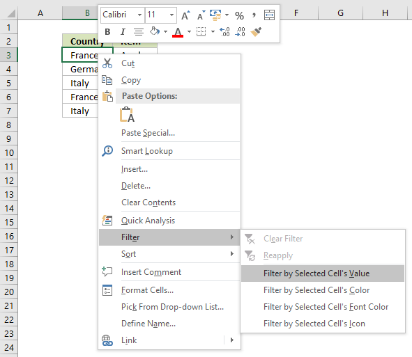
4.1 Instructions on how to filter a data set [AutoFilter]

1. Press with right mouse button on on a cell value that you want to filter
2. Press with mouse on «Filter» and then «Filter by Selected Cell’s Value»
   
3. That’s it!

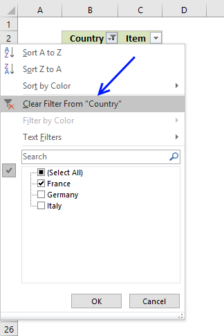
4.2 How to remove a filter

1. Press with mouse on filter button next to header, shown in picture below
   
2. Press with mouse on «Clear Filter From «Country»»
   
3. The AutoFilter buttons next to each header are still there.
   
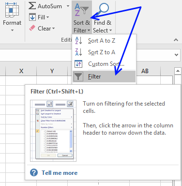
4. If you want to remove those as well, go to tab «Home» on the ribbon and press with left mouse button on «Sort & Filter» button, then on «Filter»
   
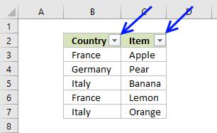
5. The data set now looks like this:
   

Back to top

5. Lookup and return multiple values [Advanced Filter]

The Advanced Filter is a tool in Excel that allows you to filter a dataset using complicated criteria combinations like AND — OR logic that the regular AutoFilter tool can’t accomplish.

In this case I am only going to filter based on a single condition so this will be an easy introduction to the Advanced Filter in Excel.

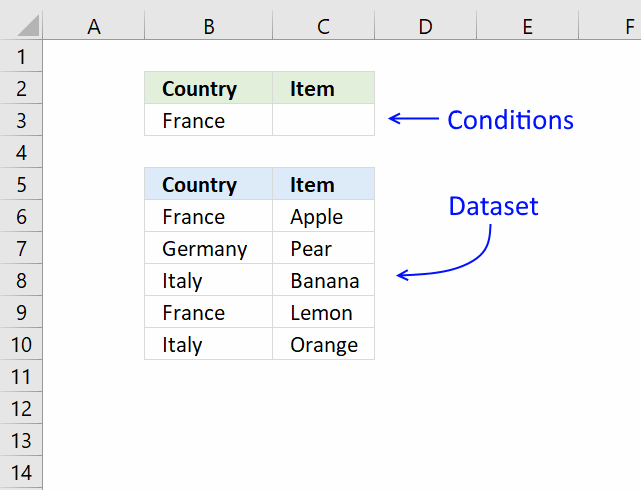
1. Copy the dataset headers and place them above or below your dataset, this to avoid confusion if the conditions disappear when a filter is applied.
   Rows will be hidden and if a condition is on the same row it will be hidden as well. I created headers on row 2, see image above.
2. Enter the condition below the correct header you want to apply a filter to, I entered my condition in cell B3.
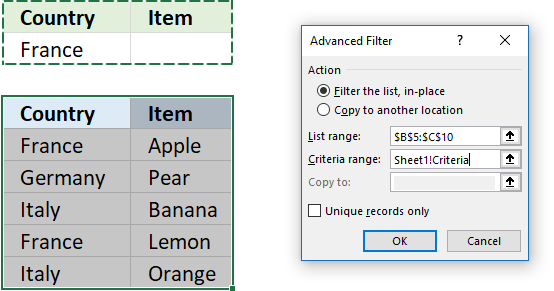
3. Select cell range B5:C10.
4. Go to tab «Data» on the ribbon.
5. Press with left mouse button on «Advanced» button.
6. Press with left mouse button on in Criteria range: field and select cell range B2:C3
   
7. Press with left mouse button on OK button.

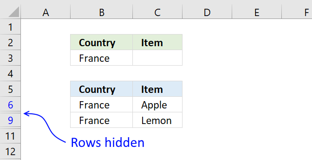
The image above shows the dataset filtered based on the condition used in cell B3. To clear the filter simply go to tab «Data» on the ribbon and press with left mouse button on «Clear» button.

Back to top

6. Lookup and return multiple values [Excel Defined Table]

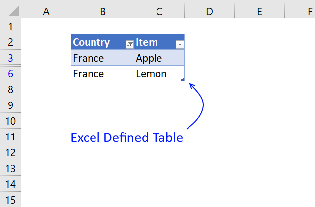
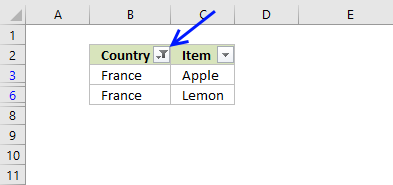
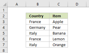
The image above shows you a dataset converted to an Excel Defined Table and filtered based on item «France» in column B.

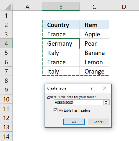
1. Select a cell in your data set.
2. Press CTRL + T (shortcut for creating an Excel Defined Table).
3. A dialog box appears, press with left mouse button on the checkbox if your data set contains headers.
   
4. Press with left mouse button on OK button.

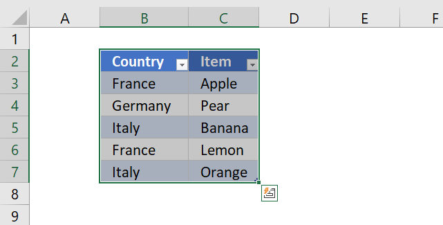
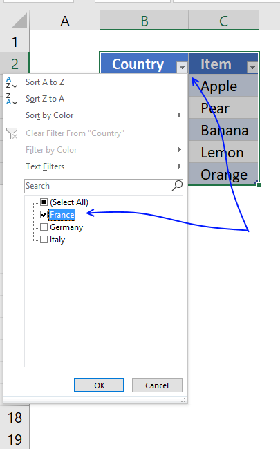
To filter the table follow these simple steps:

1. Press with left mouse button on the black arrow next to a header name.
   
2. Make sure the checkbox next to the value you want to use as a condition is selected.
3. Press with left mouse button on OK button.

So why use an Excel defined Table? An Excel defined Table contains many more useful features.

• Enter a formula in one cell and Excel automatically enters the formula in the remaining Excel Table cells on the same column.
• Cell references are converted to structured references, for example a cell reference to column «Country» might look like this: Table[Country].
  This is beneficial because you don’t need to adjust cell references if your table grows or shrinks, the cell reference is the same no matter what. You don’t need to use dynamic named ranges either.
• Easy to filter and sort data.
• Easy to add or delete data, simply type your data below the last table row and the Excel defined Table will automatically expand.
• Use as data source for a chart and the chart will display what is filtered.

Back to top

7. Return multiple values vertically or horizontally [UDF]

Make sure you have copied the vba code below into a standard module before entering the array formula.

7.1 User defined Function Syntax

vbaVlookup(lookup_value, table_array, col_index_num, [h])

7.2 Arguments

lookup_value	Required.
table_array	Required. A cell reference to the data table you want to search.
col_index_num	Required. A number representing the column in the table_array.
[h]	Optional. Return values horizontally.

Array formula in cell C14:D14:

=vbaVlookup(B14, $B$2:$C$6, 2, «h»)

7.3 Watch a video that explains how to use the User Defined Function

7.4 How to enter custom function array formula

1. Select cell range C9:C11
2. Type above custom function
3. Press and hold Ctrl + Shift
4. Press Enter once
5. Release all keys

Recommended articles

Back to top

7.5 How to enter custom function array formula

1. Select cell range C14:D14
2. Type above custom function
3. Press and hold Ctrl + Shift
4. Press Enter once
5. Release all keys

7.6 How to copy array formula to the next row

1. Select cell range C14:D14
2. Copy cell range
3. Select cell range C15:D15
4. Paste

7.7 Vba code

1. Copy vba code below.
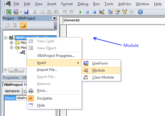
2. Press Alt + F11 to open the visual basic editor.
3. Press with right mouse button on on your workbook in the project explorer.
4. Press with mouse on «Insert».
5. Press with mouse on «Module».
   
6. Paste code to code module.
7. Exit vb editor and return to Microsoft Excel

'Name User Defined Function and arguments
Function vbaVlookup(lookup_value As Range, tbl As Range, col_index_num As Integer, Optional layout As String = "v")

'Declare variables and data types
Dim r As Single, Lrow, Lcol As Single, temp() As Variant

'Redimension array variable temp
ReDim temp(0)

'Iterate through cells in cell range
For r = 1 To tbl.Rows.Count

   'Check if lookup_value is equal to cell value
   If lookup_value = tbl.Cells(r, 1) Then

      'Save cell value to array variable temp
      temp(UBound(temp)) = tbl.Cells(r, col_index_num)

      'Add anoher container to array variable temp
      ReDim Preserve temp(UBound(temp) + 1)
   End If
Next r

'Check if variable layout equals h
If layout = "h" Then

   'Save the number of columns the user has entered this User Defined Function in. 
   Lcol = Range(Application.Caller.Address).Columns.Count
   
   'Iterate through each container in array variable temp that won't be populated
   For r = UBound(temp) To Lcol
      
       'Save a blank to array container
       temp(UBound(temp)) = ""

       'Increase the size of array variable temp with 1
       ReDim Preserve temp(UBound(temp) + 1)
   Next r

   'Decrease the size of array variable temp with 1
   ReDim Preserve temp(UBound(temp) - 1)

   'Return values to worksheet
   vbaVlookup = temp

'These lines will be rund if variable layout is not equal to h
Else

   'Save the number of rows the user has entered this User Defined Function in
   Lrow = Range(Application.Caller.Address).Rows.Count

   'Iterate through empty cells and save nothing to them in order to avoid an error being displayed
   For r = UBound(temp) To Lrow
      temp(UBound(temp)) = ""
      ReDim Preserve temp(UBound(temp) + 1)
   Next r

'Decrease the size of array variable temp with 1
ReDim Preserve temp(UBound(temp) - 1)

'Return temp variable to worksheet with values rearranged vertically
vbaVlookup = Application.Transpose(temp)
End If

End Function

Recommended reading

• Lookup multiple values in one cell [UDF]
• Fuzzy lookups [UDF]
• Filter an Excel defined Table based on selected cell [VBA]
• Filter words containing a given string in a cell range [UDF]
• Filter an Excel defined Table programmatically [VBA]
• How to save custom functions and macros to an Add-In
• Add your personal Excel Macros to the ribbon

Back to top

Back to top