Excel return the value of a cell

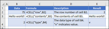
Use the CELL function to return a wide range of information about a reference. The type of information  returned is given as info_type, which must be enclosed in double quotes («»). CELL can return a cell’s address, the filename and path for a workbook, and information about the formatting used in the cell. See below for a full list of info types and format codes.

CELL is a volatile function, and can cause performance issues in large or complex worksheets.

The CELL function takes two arguments: info_type and reference. Info_type is a text string that indicates the type of information requested. See the table below for a full list of info types. Reference is a cell reference. Reference is typically a single cell. If reference refers to more than one cell, CELL returns information about the first cell in reference. For certain kinds of information (like filename) the cell address used for reference is optional and can be omitted. However, if reference is not supplied, CELL will return the name of the current «active sheet» which may or may not be the sheet where the formula exists, and might even be in a different workbook. To avoid confusion, use A1 for reference. 

Note: the CELL function is a volatile function and may cause performance issues in large or complex worksheets.

Examples

For example, to get the column number for C10:

=CELL("col", C10) // returns 3

To get the address of A1 as text:

=CELL("address",A1) // returns "$A$1"

To get the full path and workbook name for the current worksheet:

=CELL("filename",A1) // path + filename

CELL can also return format code information. For example, if A1 contains the number 100 with the currency number format applied, the CELL function will return «C2»:

=CELL("format",A1) // returns "C2"

When requesting the info_type «format» or «parentheses», a set of empty parentheses «()» is appended to the format returned if the number format uses parentheses for all values or for positive values. For example, if A1 uses the custom number format (0), then:

=CELL("format",A1) // returns "F0()"

Info types

The following info_types can be used with the CELL function:

Info_type	Description
address	returns the address of the first cell in reference (as text).
col	returns the column number of the first cell in reference.
color	returns the value 1 if the first cell in reference is formatted using color for negative values; or zero if not.
contents	returns the value of the upper-left cell in reference. Formulas are not returned. Instead, the result of the formula is returned.
filename	returns the file name and full path as text. If the worksheet that contains reference has not yet been saved, an empty string is returned.
format	returns a code that corresponds to the number format of the cell. See below for a list of number format codes. If the first cell in reference is formatted with color for values < 0, then «-» is appended to the code. If the cell is formatted with parentheses, returns «() — at the end of the code value.
parentheses	returns 1 if the first cell in reference is formatted with parentheses and 0 if not.
prefix	returns a text value that corresponds to the label prefix — of the cell:  a single quotation mark (‘) if the cell text is left-aligned, a double quotation mark («) if the cell text is right-aligned, a caret (^) if the cell text is centered text, a backslash () if the cell text is fill-aligned, and an empty string if the label prefix is anything else.
protect	returns 1 if the first cell in reference is locked or 0 if not.
row	returns the row number of the first cell in reference.
type	returns a text value that corresponds to the type of data in the first cell in reference:  «b» for blank when the cell is empty, «l»  for label if the cell contains a text constant, and «v» for value if the cell contains anything else.
width	returns the column width of the cell, rounded to the nearest integer. A unit of column width is equal to the width of one character in the default font size. Note: this value comes back as an array with two values {width,default} where width is the column width and default is a boolean value that indicates if the width is the default column width.

Format codes

The table below shows the text codes returned by CELL when «format» is used for info_type.

Format code returned	Format code meaning
G	General
F0	0
,0	#,##0
F2	0
,2	#,##0.00
C0	$#,##0_);($#,##0)
C0-	$#,##0_);[Red]($#,##0)
C2	$#,##0.00_);($#,##0.00)
C2-	$#,##0.00_);[Red]($#,##0.00)
P0	0%
P2	0.00%
S2	0.00E+00
G	# ?/? or # ??/??
D1	d-mmm-yy or dd-mmm-yy
D2	d-mmm or dd-mmm
D3	mmm-yy
D4	m/d/yy or m/d/yy h:mm or mm/dd/yy
D5	mm/dd
D6	h:mm:ss AM/PM
D7	h:mm AM/PM
D8	h:mm:ss

Notes

• The CELL function is a volatile function and may cause performance issues in large or complex worksheets.
• Reference is optional for some info types, but use an address like A1 to avoid unexpected behavior.

The CELL function returns information about the formatting, location, or contents of a cell. For example, if you want to verify that a cell contains a numeric value instead of text before you perform a calculation on it, you can use the following formula:

=IF(CELL(«type»,A1)=»v»,A1*2,0)

This formula calculates A1*2 only if cell A1 contains a numeric value, and returns 0 if A1 contains text or is blank.

Note: Formulas that use CELL have language-specific argument values and will return errors if calculated using a different language version of Excel. For example, if you create a formula containing CELL while using the Czech version of Excel, that formula will return an error if the workbook is opened using the French version.  If it is important for others to open your workbook using different language versions of Excel, consider either using alternative functions or allowing others to save local copies in which they revise the CELL arguments to match their language.

Syntax

CELL(info_type, [reference])

The CELL function syntax has the following arguments:

Argument	Description
info_type    Required	A text value that specifies what type of cell information you want to return. The following list shows the possible values of the Info_type argument and the corresponding results.
reference     Optional	The cell that you want information about. If omitted, the information specified in the info_type argument is returned for cell selected at the time of calculation. If the reference argument is a range of cells, the CELL function returns the information for active cell in the selected range. Important: Although technically reference is optional, including it in your formula is encouraged, unless you understand the effect its absence has on your formula result and want that effect in place. Omitting the reference argument does not reliably produce information about a specific cell, for the following reasons: In automatic calculation mode, when a cell is modified by a user the calculation may be triggered before or after the selection has progressed, depending on the platform you’re using for Excel.  For example, Excel for Windows currently triggers calculation before selection changes, but Excel for the web triggers it afterward. When Co-Authoring with another user who makes an edit, this function will report your active cell rather than the editor’s. Any recalculation, for instance pressing F9, will cause the function to return a new result even though no cell edit has occurred.

info_type values

The following list describes the text values that can be used for the info_type argument. These values must be entered in the CELL function with quotes (» «).

info_type	Returns
«address»	Reference of the first cell in reference, as text.
«col»	Column number of the cell in reference.
«color»	The value 1 if the cell is formatted in color for negative values; otherwise returns 0 (zero). Note: This value is not supported in Excel for the web, Excel Mobile, and Excel Starter.
«contents»	Value of the upper-left cell in reference; not a formula.
«filename»	Filename (including full path) of the file that contains reference, as text. Returns empty text («») if the worksheet that contains reference has not yet been saved. Note: This value is not supported in Excel for the web, Excel Mobile, and Excel Starter.
«format»	Text value corresponding to the number format of the cell. The text values for the various formats are shown in the following table. Returns «-» at the end of the text value if the cell is formatted in color for negative values. Returns «()» at the end of the text value if the cell is formatted with parentheses for positive or all values. Note: This value is not supported in Excel for the web, Excel Mobile, and Excel Starter.
«parentheses»	The value 1 if the cell is formatted with parentheses for positive or all values; otherwise returns 0. Note: This value is not supported in Excel for the web, Excel Mobile, and Excel Starter.
«prefix»	Text value corresponding to the «label prefix» of the cell. Returns single quotation mark (‘) if the cell contains left-aligned text, double quotation mark («) if the cell contains right-aligned text, caret (^) if the cell contains centered text, backslash () if the cell contains fill-aligned text, and empty text («») if the cell contains anything else. Note: This value is not supported in Excel for the web, Excel Mobile, and Excel Starter.
«protect»	The value 0 if the cell is not locked; otherwise returns 1 if the cell is locked. Note: This value is not supported in Excel for the web, Excel Mobile, and Excel Starter.
«row»	Row number of the cell in reference.
«type»	Text value corresponding to the type of data in the cell. Returns «b» for blank if the cell is empty, «l» for label if the cell contains a text constant, and «v» for value if the cell contains anything else.
«width»	Returns an array with 2 items. The 1st item in the array is the column width of the cell, rounded off to an integer. Each unit of column width is equal to the width of one character in the default font size. The 2nd item in the array is a Boolean value, the value is TRUE if the column width is the default or FALSE if the width has been explicitly set by the user.  Note: This value is not supported in Excel for the web, Excel Mobile, and Excel Starter.

CELL format codes

The following list describes the text values that the CELL function returns when the Info_type argument is «format» and the reference argument is a cell that is formatted with a built-in number format.

If the Excel format is	The CELL function returns
General	«G»
0	«F0»
#,##0	«,0»
0.00	«F2»
#,##0.00	«,2»
$#,##0_);($#,##0)	«C0»
$#,##0_);[Red]($#,##0)	«C0-«
$#,##0.00_);($#,##0.00)	«C2»
$#,##0.00_);[Red]($#,##0.00)	«C2-«
0%	«P0»
0.00%	«P2»
0.00E+00	«S2»
# ?/? or # ??/??	«G»
m/d/yy or m/d/yy h:mm or mm/dd/yy	«D4»
d-mmm-yy or dd-mmm-yy	«D1»
d-mmm or dd-mmm	«D2»
mmm-yy	«D3»
mm/dd	«D5»
h:mm AM/PM	«D7»
h:mm:ss AM/PM	«D6»
h:mm	«D9»
h:mm:ss	«D8»

Note: If the info_type argument in the CELL function is «format» and you later apply a different format to the referenced cell, you must recalculate the worksheet (press F9) to update the results of the CELL function.

Examples

Need more help?

You can always ask an expert in the Excel Tech Community or get support in the Answers community.

See Also

Change the format of a cell

Create or change a cell reference

ADDRESS function

Add, change, find or clear conditional formatting in a cell

This Tutorial demonstrates how to use the Excel CELL Function in Excel to get information about a cell.

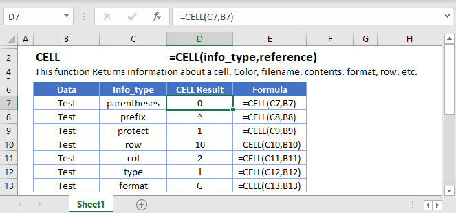
CELL Function Overview

The CELL Function Returns information about a cell. Color, filename, contents, format, row, etc.

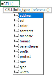
To use the CELL Excel Worksheet Function, select a cell and type:

(Notice how the formula inputs appear)

CELL function Syntax and inputs:

=CELL(info_type,reference)

info_type – Text indicating what cell information you would like to return.

reference – The cell reference that you want information about.

How to use the CELL Function in Excel

The CELL Function returns information about the formatting, location, or contents of cell.

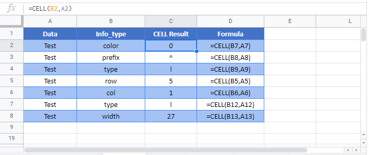
=CELL(D3,$B$3)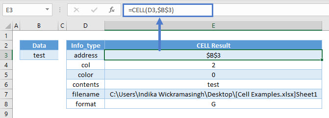

As seen above, the CELL Function returns all kinds of information from cell B3.

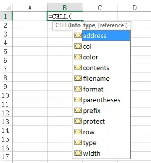
If you type =CELL(, you will be able to see 12 different types of information to retrieve.

Here are additional outputs of the CELL Function:

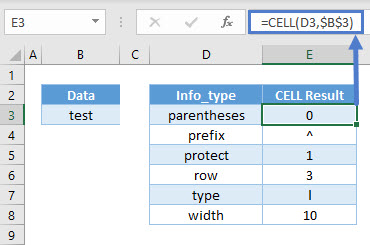
Overall View of Info_types

Some of the info_types are pretty straightforward and retrieves what you asked for, while the rest will be explained in the next few sections because of the complexity.

Info_type	What it retrieves?
“address”	The cell reference/address.
“col”	The column number.
“color”	*
“contents”	The value itself or result of the formula.
“filename”	The full path, filename, and extension in square brackets, and sheet name.
“format”	*
“parentheses”	*
“prefix”	*
“protect”	*
“row”	The row number.
“type”	*
“width”	The column width rounded to the nearest integer.

* Explained in the next few sections.

Color Info_type

Color will show all results as 0 unless the cell is formatted with color for negative values. The latter will show as 1.

=CELL("color",B3)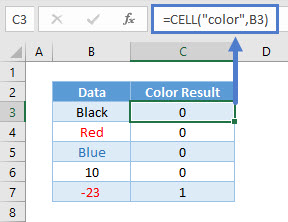

Format Info_type

Format shows the number format of the cell, but it might not be what you expect.

=CELL("format",B3)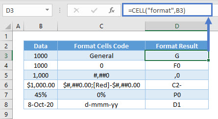

There are many kinds of different variations with formatting, but here are some guidelines to figure it out:

• “G” is for General, “C” for Currency, “P” for Percentage, “S” for Scientific (not shown above), “D” for Date.
• If the digits are with numbers, currencies, and percentages; it represents the decimal places. Eg. “F0” means 0 decimals in cell D4, and “C2-” means 2 decimals in cell D6. “D1” in cell D8 is simply a type of date format (there are D1 to D9 for different kinds of date and time formats).
• A comma at the beginning is for thousand separators (“,0” in cell D5 for eg).
• A minus sign is for formatting negative values with a color (“C2-” in cell D6 for eg).

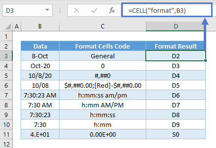
Here are other examples of date formats and for scientific.

Parentheses Info_type

Parentheses shows 1 if the cell is formatted with parentheses (either or both positive and negative). Otherwise, it shows 0.

=CELL("parentheses",B3)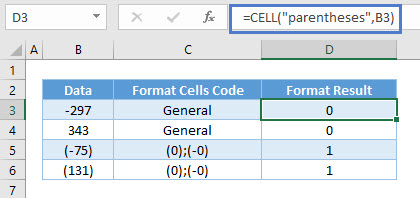

Prefix Info_type

Prefix results in various symbols depending on how the text is aligned in the cell.

=CELL("prefix",B3)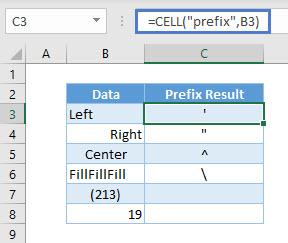

As seen above, a left alignment of the text is a single quote in cell C3.
A right alignment of the text shows double quotes in cell C4.
A center alignment of the text shows caret in cell C5.
A fill alignment of the text shows backslash in cell C6.
Numbers (cell C7 and C8) show as blank regardless of alignment.

Protect Info_type

Protect results in 1 if the cell is locked, and 0 if it’s unlocked.

=CELL("protect",B3)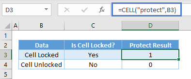

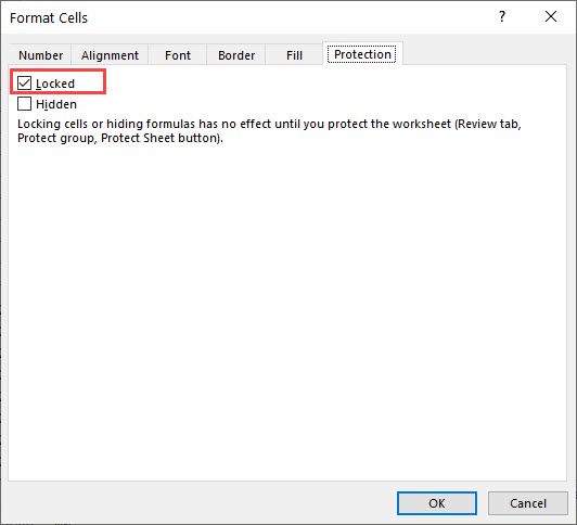
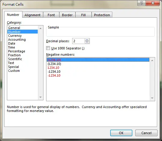
Do note that all cells are locked by default. That is why you can’t edit any cells after you protect it. To unlock it, right-click on a cell and choose Format Cells.

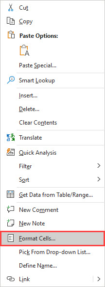
Go to the Protection tab and you can uncheck “Locked” to unlock the cell.

Type Info_type

Type results in three different alphabets dependent on the data type in the cell.

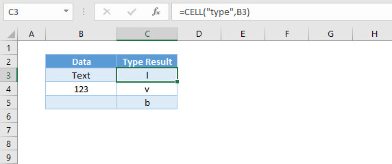
“l” stands for label in cell C3.
“v” stands for value in cell C4.
“b” stands for blank in cell C5.

Create Hyperlink to Lookup Using Address

You can use the CELL Function along with HYPERLINK and INDEX / MATCH to hyperlink to a lookup result:

=HYPERLINK("#"&CELL("address",INDEX(C3:C6,MATCH("mango",B3:B6,0))),INDEX(C3:C6,MATCH("mango",B3:B6,0)))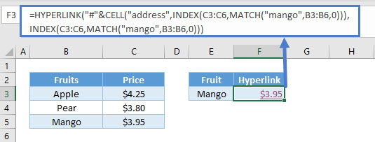

The INDEX and MATCH formula retrieves the price of Mango in cell C5: $3.95. The CELL Function, with “address” returns the cell location. The HYPERLINK function then creates the hyperlink.

Retrieve File Path

To retrieve the file path where the particular file is stored, you can use:

=LEFT(CELL("filename"),FIND("[",CELL("filename"))-1)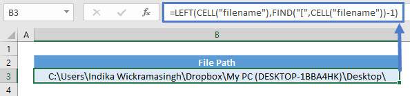

Since the filename will be the same using any cell reference, you can omit it. Use FIND function to obtain the position where “[“ starts and minus 1 to allow LEFT function to retrieve the characters before that.

Retrieve File Name

To retrieve the file name, you can use:

=MID(CELL("filename"),FIND("[",CELL("filename"))+1,FIND("]",CELL("filename"))-FIND("[",CELL("filename"))-1)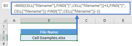

This uses a similar concept as above where FIND function obtains the position where “[“ starts and retrieves the characters after that. To know how many characters to extract, it uses the position of “]” minus “[“ and minus 1 as it includes the position of “]”.

Retrieve Sheet Name

To retrieve the sheet name, you can use:

=MID(CELL("filename"),FIND("]",CELL("filename"))+1,LEN(CELL("filename")))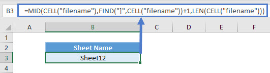

Again, it’s similar to the above where FIND function obtains the position where “]“ starts and retrieves the characters after that. To know how many characters to extract, it uses the total length of what “filename” info_type returns.

CELL Function in Google Sheets

The CELL function works similarly in Google Sheets. It just doesn’t have the full range of info_type. It only includes “address”, “col”, “color”, “contents”, “prefix”, “row”, “type”, and “width”.

Additional Notes

The CELL Function returns information about a cell. The information that can be returned relates to cell location, formatting and contents.

Enter the type of information you want then enter the cell reference for the cell you want information about.

Return to the List of all Functions in Excel

This Excel tutorial explains how to use Cell Function to check Cell format, address and contents.

You may also want to read:

Excel ColorIndex Property

Excel verify Number format and convert Text to Number

Excel Cell Function is a very powerful Function that tells various information of a Cell. Cell Function has a list of arguments regarding Cell information.

Syntax of Cell Function

CELL(info_type, [reference])

[reference] is the Cell you want to get information from, only one Cell is expected. If you enter multiple Range, only information of the top left Cell will return.

info_type	Explanation
“address”	Return Absolute Address of a Cell
“col”	Return column number of a Cell
“color”	Returns 1 if the Cell is formatted to change color font for negative value; Otherwise it returns 0
“contents”	Return Value of a Cell
“filename”	Filename (including full path) of the file that contains reference, as text. Returns empty text (“”) if the worksheet that contains reference has not yet been saved.
“format”	Return Number format of the cell. You are required to recalculate the formula (double click the formula Cell and then exit edit) when the format is changed. If the Excel format is The CELL function returns General “G” 0 “F0” #,##0 “,0” 0.00 “F2” #,##0.00 “,2” $#,##0_);($#,##0) “C0” $#,##0_);[Red]($#,##0) “C0-“ $#,##0.00_);($#,##0.00) “C2” $#,##0.00_);[Red]($#,##0.00) “C2-“ 0% “P0” 0.00% “P2” 0.00E+00 “S2” # ?/? or # ??/?? “G” m/d/yy or m/d/yy h:mm or mm/dd/yy “D4” d-mmm-yy or dd-mmm-yy “D1” d-mmm or dd-mmm “D2” mmm-yy “D3” mm/dd “D5” h:mm AM/PM “D7” h:mm:ss AM/PM “D6” h:mm “D9” h:mm:ss “D8”
“parentheses”	Returns 1 if the cell is formatted with parentheses; Otherwise, it returns 0.
“prefix”	Label prefix for the cell. * Returns a single quote (‘) if the cell is left-aligned. * Returns a double quote (“) if the cell is right-aligned. * Returns a caret (^) if the cell is center-aligned. * Returns a back slash () if the cell is fill-aligned. * Returns an empty text value for all others.
“protect”	Returns 1 if the cell is locked. Returns 0 if the cell is not locked.
“row”	Row number of the cell.
“type”	Returns “b” if the cell is empty. Returns “l” if the cell contains a text constant. Returns “v” for all others.
“width”	Column width of the cell, rounded to the nearest integer.

Example of Cell Function

Some of the info_type are self-explanatory, and more importantly they are rarely used, so I am not going to go through each of them.

The most important use of Cell Function includes Address, Row and Column. See the examples below.

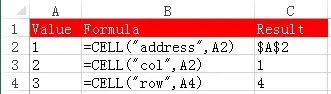
You may use Substitute Function to get rid of the $ in absolute address.

=Substitute(CELL("address",A2),"$","")

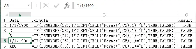
The second most important use of Cell Function is to check whether a Cell contains a Date.

Since a Date is a serial number, from Excel’s perspective, Date is regarded as number. The only difference between a Date and Number is how it is formatted. Therefore to tell the difference between a Date and a Number, we should use info_type “format” and see if the returned value starts with “D”.

The following formula returns TRUE if it is a Date

=IF(ISNUMBER(A2),IF(LEFT(CELL("Format",A2),1)="D",TRUE,FALSE))

Misuse of Cell Function

One important point to note is that the info_type “color” is not to detect color of the Cell, it is just a checking whether you have formatted to number to change color for negative number.

If you want to check the color of the Cell, use ColorIndex Property

Outbound References

https://support.office.com/en-ca/article/CELL-function-51bd39a5-f338-4dbe-a33f-955d67c2b2cf

In this article, we will learn about how to get the cell value at a given row and column number in Excel.

To get the cell value you need to know the address of the cell. But here we have the Row & column number of the cell where our required value is. So we use a combination of INDIRECT function & ADDRESS function to get the cell value.

The INDIRECT function is a cell reference function. It takes the value in the cell as address and returns the value in the address cell.

Syntax:

The ADDRESS function simply returns the address of a cell by using row number and column number.

Syntax:

= ADDRESS ( row_num , col_num )

Let’s make a formula using the above functions:
Firstly, we can get the address of the function as ADDRESS function returns the address of the cell using row & column number. And then Indirect function extracts out the cell value from the address returned by the address function.
Syntax:

Let’s understand this function using it in an example.

Here we have table_array and Row & Column number in the right of the below snapshot.

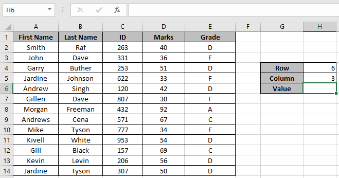
We need to find the cell value in 6th row and 3rd column

Use the formula:

Explanation:
ADDRESS ( H4 , H5 ) returns $C$6 (address to the required cell).
The INDIRECT ($C$6) returns the cell value at C6 cell.

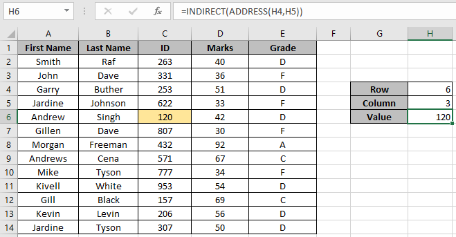
As you can see the formula returns the value for a given row & column number.

Notes:

1. The function returns an error if the address returned by the ADDRESS function is not valid.
2. The function returns 0 if the cell value is blank.
3. Use the INDEX function as INDIRECT function is a volatile function.

That’s all about, how to get the cell value at a given row and column number in Excel. Explore more articles on Excel Formulas here. Please feel free to state your query or feedback for the above article.

Related Articles
How to use the INDIRECT function in Excel

How to use the ADDRESS function in Excel

How to use the VLOOKUP function in Excel

How to use the HLOOKUP function in Excel

17 Things About Excel VLOOKUP

Popular Articles
Edit a dropdown list

If with conditional formatting

If with wildcards

Vlookup by date