
Required Rate of Return Formula (Table of Contents)
- Required Rate of Return Formula
- Examples of Required Rate of Return Formula (With Excel Template)
- Required Rate of Return Formula Calculator
Required Rate of Return Formula
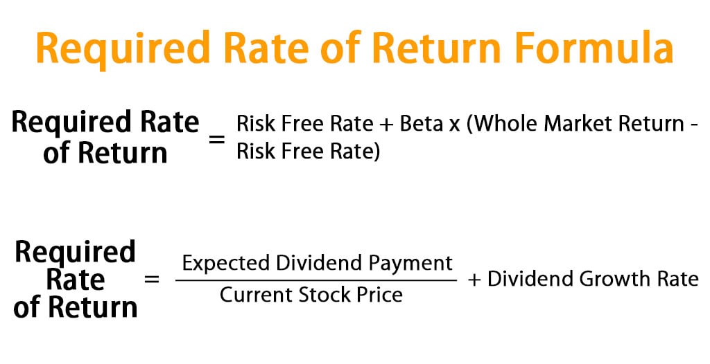
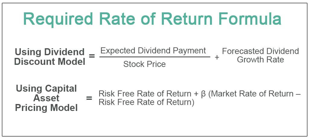
The Required return is a minimum return or profit what an investor expects from doing business or buying stocks with respect to the risks associated with it for running a business or holding the stocks. It can otherwise be called Hurdle Rate. This is the minimum return an investor required for compensating the level of risk associated. Riskier projects have high return meanwhile less risky have low returns. Both Returns and risk are directly proportional to each other. So based on the tolerance over the risk by the investor, the required rate of return May change. This factor is mostly considered in stock markets. The formula acts as a decision maker as it calculates how much minimum Return an investor can expect by investing for a company. The Required Rate of Return Formula can be calculated using “Capital Asset Pricing Model (CAPM)” which is widely used where there are no dividends. However this method considers some factors while assessing, it considers some factors such as, assume that you took the stock with no risk, the whole market return, and overall cost of funding a project (Beta). The Mathematical formula for the required rate of Return is,
Required Rate of Return = Risk Free Rate + Beta * (Whole Market Return – Risk Free Rate)
Alternatively, the required rate of Return can also be calculated using the Dividend Discount Approach (known as ‘Gordon Growth Model’) where Dividend takes place. This Formula considers certain factors such as current stock price, Dividend growth at a constant rate, dividend payment. It is mathematically represented as,
Required Rate of Return = (Expected Dividend Payment / Current Stock Price) + Dividend Growth Rate
Examples of Required Rate of Return Formula (With Excel Template)
Let’s take an example to understand the calculation of the Required Rate of Return formula in a better manner.
You can download this Required Rate of Return Formula Excel Template here – Required Rate of Return Formula Excel Template
Required Rate of Return Formula – Example #1
CAPM:
Here is an example to calculate the required rate of return for an investor to invest in a company called XY Limited which is a food processing company. Let us assume the beta value is 1.30. The risk free rate is 5%. The whole market return is 7%.
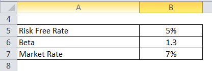
Required Rate of Return is calculated using the formula given below
Required Rate of Return = Risk Free Rate + Beta * (Whole Market Return – Risk Free Rate)
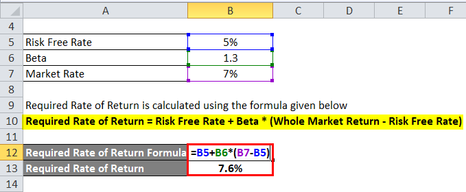
- Required Rate of Return = 5% + 1.3 * (7% – 5%)
- Required Rate of Return = 7.6%
Dividend Discount Model:
For this model consider XY Limited is paying dividends of Rs.140 per stock. The dividend growth rate is 7%. The current stock price is RS.200.
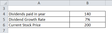
Required Rate of Return is calculated using the formula given below
Required Rate of Return = (Expected Dividend Payment / Current Stock Price) + Dividend Growth Rate
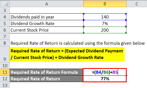
- Required Rate of Return = (140 / 200) + 7%
- Required Rate of Return = 77%
Required Rate of Return Formula – Example #2
CAPM:
Let us take the real-life example of Tata Group of company with the following information available.
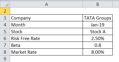
Required Rate of Return is calculated using the formula given below
Required Rate of Return = Risk Free Rate + Beta * (Whole Market Return – Risk Free Rate)
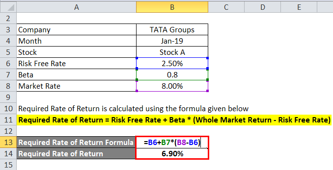
- Required Rate of Return = 2.50% + 0.8 * (8% – 2.50%)
- Required Rate of Return = 6.90%
Dividend Discount model:
Let us take the real-life example of Tata Group of company with the following information available.
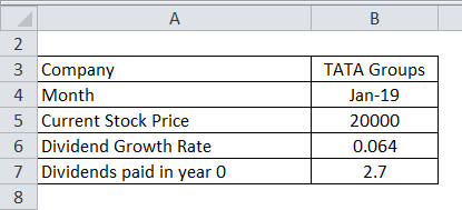
Required Rate of Return is calculated using the formula given below
Required Rate of Return = (Expected Dividend Payment / Current Stock Price) + Dividend Growth Rate
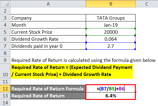
- Required Rate of Return = (2.7 / 20000) + 0.064
- Required Rate of Return = 6.4 %
Explanation of Required Rate of Return Formula
- CAPM: Here is the step by step approach for calculating Required Return.
Step 1: Theoretically RFR is risk free return is the interest rate what an investor expects with zero Risk. Practically any investments you take, it at least carries a low risk so it is not possible with zero risk rate. In India, the government 10 years bond interest rate is around 6% (least Risk rate) can be taken for this benchmark.
Step 2: β is the Beta coefficient value of Stocks which is the measure of the volatility in comparison to the market or benchmark. It is the tendency of a return to respond to swing in the market. That is how much risk investment will add to the portfolio in the market. This can be computed by dividing the covariance of the Asset and Market return’s product by the product of the variance of the Market.
Beta = Covariance (Return of the Asset * Return of the Market) / Variance (Return of the Market)
Good Beta value is 1 as per the standard index. Beta with lesser than 1 has a low risk as well as low returns. A beta value greater than 1 has a high risk and high yield.
Step 3: Whole Market Return is the return expected from the market. You can get the market return by searching in the net or you can refer the standard index such as NIFTY 50 index.
Step 4: Finally, the Required rate of return is got by applying the values which were forecasted as shown below.
Required Rate of Return = Risk-Free Rate + Beta * (Whole Market Return – Risk-Free Rate)
- Dividend Discount Model: On the other hand, the following steps help in calculating the required rate of return by using the alternate method. This model is only applicable when a company has a stable dividend per stock rate.
Step 1: Firstly, the Expected dividend payment is the payment expected to be paid next year.
Step 2: Current stock price. If you are using the newly issued common stock, you will have to minus the floating costs from it.
Step 3: The Growth rate of the dividend is the stable dividend rate a company has over a period of time.
Step 4: Finally, the required rate of return is calculated by applying these values in the below formula.
Required Rate of Return = (Expected Dividend Payment / Current Stock Price) + Dividend Growth Rate
Relevance and Uses of Required Rate of Return Formula
The required rate of return formula is a key term in equity and corporate finance. Investment decisions are not only limited to Share markets. Whenever the money is invested in a business or for business expansion, an analyst looks at the minimum return expected for taking the risks. These decisions are the core reasons for multiple investments. So it calculates the present dividend income value while evaluating stocks. As well as, it calculates the present free cash flow into equity. For capital projects, it helps to determine whether to pursue one project versus another or not. It is the minimum return amount, an investor considers acceptable with respect to its capital cost, inflation, and yield on other projects.
Required Rate of Return Formula Calculator
You can use the following Required Rate of Return Calculator.
| Risk Free Rate | |
| Beta | |
| Whole Market Return | |
| Required Rate of Return Formula = | |
| Required Rate of Return Formula = | Risk Free Rate + Beta x (Whole Market Return — Risk Free Rate) |
| = |
0 + 0 x (0 — 0) = 0 |
Recommended Articles
This has been a guide to Required Rate of Return formula. Here we discuss How to Calculate Required Rate of Return along with practical examples. We also provide the Required Rate of Return Calculator with downloadable excel template. You may also look at the following articles to learn more –
- Formula for Break Even Analysis
- Calculation of Discount Factor
- Calculate Simple Interest Rate using Formula
- Examples of Price Index Formula
- How to Calculate Risk Free Rate Formula?
- Dividend Discount Model with Examples
What is the Required Rate of Return Formula?
The formula for calculating the required rate of return for stocks paying a dividend is derived using the Gordon growth modelGordon Growth Model is a Dividend Discount Model variant used for stock price calculation as per the Net Present Value (NPV) of its future dividends. read more. This dividend discount model calculates the required return for equity of a dividend-paying stock by using the current stock price, the dividend payment per share, and the expected dividend growth rate.
The formula using the dividend discount modelThe Dividend Discount Model (DDM) is a method of calculating the stock price based on the likely dividends that will be paid and discounting them at the expected yearly rate. In other words, it is used to value stocks based on the future dividends’ net present value.read more is represented as,
Required Rate of Return formula = Expected dividend payment / Stock price + Forecasted dividend growth rate
The required return equation utilizes the risk-free rate of return and the market rate of return, typically the benchmark index’s annual return. On the other hand, calculating the required rate of return for stock not paying a dividend is derived using the Capital Asset Pricing ModelThe Capital Asset Pricing Model (CAPM) defines the expected return from a portfolio of various securities with varying degrees of risk. It also considers the volatility of a particular security in relation to the market.read more (CAPM). The CAPM method calculates the required return by using the beta of security, which is the indicator of the riskiness of that security.
The formula using the CAPM method is represented as,
Required Rate of Return formula = Risk-free rate of return + β * (Market rate of return – Risk-free rate of return)
Table of contents
- What is the Required Rate of Return Formula?
- Steps to Calculate Required Rate of Return using the Dividend Discount Model
- Steps to Calculate Required Rate of Return using CAPM Model
- Examples of Required Rate of Return Formula (with Excel Template)
- Example #1
- Example #2
- Relevance and Uses
- Recommended Articles
Steps to Calculate Required Rate of Return using the Dividend Discount Model
For stock paying a dividend, the required rate of return (RRR) formula can be calculated by using the following steps:
- Firstly, determine the dividend to be paid during the next period.
- Next, gather the current price of the equity from the stock.
- Now, try to figure out the expected growth rate of the dividend based on management disclosure, planning, and business forecast.
- Finally, the required rate return is calculated by dividing the expected dividend payment (step 1) by the current stock price (step 2) and then adding the result to the forecasted dividend growth rate (step 3) as shown below,
Required rate of return formula = Expected dividend payment / Stock price + Forecasted dividend growth rate
Steps to Calculate Required Rate of Return using CAPM Model
The required rate of return for a stock not paying any dividend can be calculated by using the following steps:
Step 1: Firstly, determine the risk-free rate of return, which is the return of any government issues bonds such as 10-year G-Sec bonds.
Step 2: Next, determine the market rate of return, the annual return of an appropriate benchmark index such as the S&P 500 index. The market risk premium can be calculated by deducting the risk-free return from the market return.
Market risk premium = Market rate of return – Risk-free rate of return
Step 3: Next, compute the stock’s beta based on its stock price movement vis-à-vis the benchmark index.
Step 4: Finally, the required rate of return is calculated by adding the risk-free rate to the product of beta and market risk premiumThe market risk premium is the supplementary return on the portfolio because of the additional risk involved in the portfolio; essentially, the market risk premium is the premium return investors should have to make sure to invest in stock instead of risk-free securities.read more (step 2) as given below,
The required rate of return formula = Risk-free rate of return + β * (Market rate of return – Risk-free rate of return)
Examples of Required Rate of Return Formula (with Excel Template)
Let’s see some simple to advanced examples to understand the calculation of the Required Rate of Return better.
You can download this Required Rate of Return Formula Excel Template here – Required Rate of Return Formula Excel Template
Example #1
Let us take an example of an investor considering two securities of equal risk to include one of them in his portfolio.
Determine which security should be selected based on the following information:
Below is data for calculation of the required rate of return for Security A and Security B.
| Particulars | Security A | Security B |
|---|---|---|
| Expected Dividend | $10 | $8 |
| Current Stock Price | $160 | $100 |
| Forecasted Dividend Growth Rate | 5% | 4% |
The required return of security A can be calculated as,
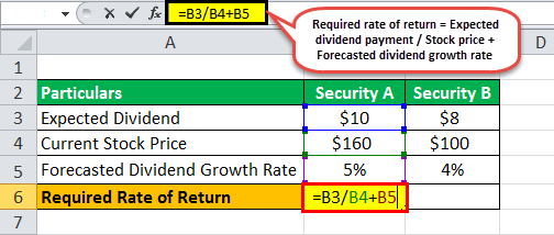
Required return for security A = $10 / $160 * 100% + 5%
The required return for security A= 11.25%
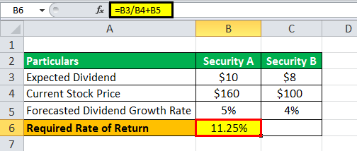
The required return of security B can be calculated as,
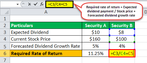
Required return for security B = $8 / $100 * 100% + 4%
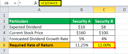
The required return for security B = 12.00%
Based on the given information, Security A should be preferred for the portfolio because its lower required return gave the risk level.
Example #2
Calculate the required rate of return of the stock based on the given information. Let us take an example of a stock with a beta of 1.75, i.e., it is riskier than the overall market. Further, the US treasury bond’s short-term return stood at 2.5%, while the benchmark index is characterized by a long-term average return of 8%.
- Given, Risk-free rate = 2.5%
- Beta = 1.75
- Market rate of return = 8%
Below is data for the calculation of a required rate of return of the stock-based.
| Risk Free Rate | 2.50% |
| Beta of the Stock | 1.75 |
| Market Rate of Return | 8.00% |
Therefore, the required return of the stock can be calculated as,
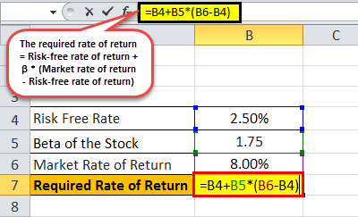
Required return = 2.5% + 1.75 * (8% – 2.5%)
= 12.125%
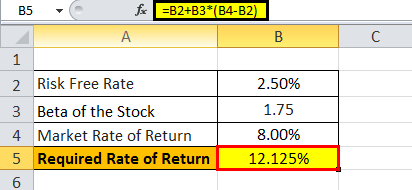
Therefore, the required return of the stock is 12.125%.
Relevance and Uses
It is important to understand the concept of the required return as investors use it to decide on the minimum amount of return required from an investment. Based on the required returns, an investor can decide whether to invest in an asset based on the given risk level.
The required return for a stock with a high beta relative to the market should have been higher because it is necessary to compensate investors for the added risk associated with the investment. Also, an investor can use the required returns for ranking the assets and eventually make the investment as per the ranking and include them in the portfolio. In short, the higher the expected return, the better is the asset.
Recommended Articles
This article has been a guide to the Required Rate of Return Formula. Here we discuss how to calculate the Required Rate of Return using practical examples and downloadable excel templates. You may learn more about Valuation from the following articles –
- Calculate Market Risk PremiumMarket risk premium refers to the extra return expected by an investor for holding a risky market portfolio instead of risk-free assets. Market risk premium = expected rate of return – risk free rate of returnread more
- Rate of Return FormulaRate of Return (ROR) refers to the expected return on investment (gain or loss) & it is expressed as a percentage. You can calculate this by, ROR = {(Current Investment Value – Original Investment Value)/Original Investment Value} * 100read more
- Expected Return Calculation
- Cash on Cash Return
What Is the Internal Rate of Return (IRR)?
The internal rate of return (IRR) is the discount rate providing a net value of zero for a future series of cash flows. Both the IRR and net present value (NPV) are used when selecting investments based on their returns.
Excel has three functions for calculating the internal rate of return that include Internal Rate of Return (IRR), Modified Internal Rate of Return (MIRR), and Internal Rate of Return with time periods (XIRR).
The IRR function calculates the internal rate of return for a series of cash flows, the MIRR function works with interest rates for borrowing and investing, and the XIRR function calculates a more accurate internal rate of return as it considers time periods.
Key Takeaways
• The internal rate of return (IRR) is the discount rate providing a net value of zero for a future series of cash flows.
• Excel has three functions for calculating the internal rate of return.
• When using different borrowing rates of reinvestment, a modified internal rate of return (MIRR) applies.
• The XIRR function accounts for different time periods.
How to Calculate IRR in Excel
What Is Net Present Value?
NPV is the difference between the present value of cash inflows and the present value of cash outflows over time.
The net present value of a project depends on the discount rate used. So when comparing two investment opportunities, the choice of the discount rate, which is often based on a degree of uncertainty, will have a considerable impact.
In the example below, using a 20% discount rate, investment #2 shows higher profitability than investment #1. When opting instead for a discount rate of 1%, investment #1 shows a return bigger than investment #2. Profitability often depends on the sequence and importance of the project’s cash flow and the discount rate applied to those cash flows.
How IRR and NPV Differ
The main difference between the IRR and NPV is that NPV is an actual amount while the IRR is the interest yield as a percentage expected from an investment.
Investors typically select projects with an IRR that is greater than the cost of capital. However, selecting projects based on maximizing the IRR as opposed to the NPV could result in suboptimal economic outcomes.
IRR represents the actual annual return on investment only when the project generates zero interim cash flows, or if those investments can be invested at the current IRR.
Calculating IRR in Excel
The IRR is the discount rate that can bring an investment’s NPV to zero. When the IRR has only one value, this criterion becomes more interesting when comparing the profitability of different investments.
In our example, the IRR of investment #1 is 48% and, for investment #2, the IRR is 80%. This means that in the case of investment #1, with an investment of $2,000 in 2013, the investment will yield an annual return of 48%. In the case of investment #2, with an investment of $1,000 in 2013, the yield will bring an annual return of 80%.
If no parameters are entered, Excel starts testing IRR values differently for the entered series of cash flows and stops as soon as a rate is selected that brings the NPV to zero. If Excel does not find any rate reducing the NPV to zero, it shows the error «#NUM.»
If the second parameter is not used and the investment has multiple IRR values, we will not notice because Excel will only display the first rate it finds that brings the NPV to zero.
In the image below, for investment #1, Excel does not find the NPV rate reduced to zero, so we have no IRR.
The image below also shows investment #2. If the second parameter is not used in the function, Excel will find an IRR of -10%. On the other hand, if the second parameter is used (i.e., = IRR ($ C $ 6: $ F $ 6, C12)), there are two IRRs rendered for this investment, which are -10% and 216%.
If the cash flow sequence has only a single cash component with one sign change (from + to — or — to +), the investment will have a unique IRR. However, most investments begin with a negative flow and a series of positive flows as the first investments come in. Profits then, hopefully, subside, as was the case in our first example.
In the image below, we calculate the IRR. To do this, we simply use the Excel IRR function:
Calculating MIRR in Excel
When a company uses different borrowing rates of reinvestment, the modified internal rate of return (MIRR) applies.
In the image below, we calculate the IRR of the investment as in the previous example but taking into account that the company will borrow money to plow back into the investment (negative cash flows) at a rate different from the rate at which it will reinvest the money earned (positive cash flow). The range C5 to E5 represents the investment’s cash flow range, and cells D10 and D11 represent the rate on corporate bonds and the rate on investments.
The image below shows the formula behind the Excel MIRR. We calculate the MIRR found in the previous example with the MIRR as its actual definition. This yields the same result: 56.98%.
(
−
NPV
(
rrate, values
[
positive
]
)
×
(
1
+
rrate
)
n
NPV
(
frate, values
[
negative
]
)
×
(
1
+
frate
)
)
1
n
−
1
−
1
begin{aligned}left(frac{-text{NPV}(textit{rrate, values}[textit{positive}])times(1+textit{rrate})^n}{text{NPV}(textit{frate, values}[textit{negative}])times(1+textit{frate})}right)^{frac{1}{n-1}}-1end{aligned}
(NPV(frate, values[negative])×(1+frate)−NPV(rrate, values[positive])×(1+rrate)n)n−11−1
Calculating XIRR in Excel
The XIRR function takes into consideration different periods. To use this function, Excel requires both the cash flow amounts as well as the dates on which those cash flows are paid.
In the example below, the cash flows are not disbursed at the same time each year – as is the case in the above examples. Rather, they are happening at different periods. We use the XIRR function below to solve this calculation. We first select the cash flow range (C5 to E5) and then select the range of dates on which the cash flows are realized (C32 to E32).
For investments with cash flows received or cashed at different moments in time for a firm that has different borrowing rates and reinvestments, Excel does not provide functions that can be applied to these situations although they are probably more likely to occur.
Q. I have prepared projections for a proposed project, and I want to calculate the internal rate of return. Instead of using Excel’s IRR function, should I use simple math formulas so others can follow my calculations?
A. Excel offers three functions for calculating the internal rate of return, and I recommend you use all three. The problem with using math to calculate the internal rate of return is that the necessary calculations are both complicated and time—consuming. Basically, a math—based solution involves calculating the net present value (NPV) for each cash flow amount (in a series of cash flows) using various guessed interest rates on a trial—and—error basis, and then those NPVs are added together. This process is repeated using various interest rates until you find/stumble upon the exact interest rate that produces NPV amounts that sum to zero. The interest rate that produces a zero—sum NPV is then declared the internal rate of return.
To simplify this process, Excel offers three functions for calculating the internal rate of return, each of which represents a better option than using the math—based formulas approach. These Excel functions are IRR, XIRR, and MIRR. Explanations and examples for these functions are presented below. You can download the example workbook at carltoncollins.com/irr.xlsx.
1. Excel’s IRR function. Excel’s IRR function calculates the internal rate of return for a series of cash flows, assuming equal-size payment periods. Using the example data shown above, the IRR formula would be =IRR(D2:D14,.1)*12, which yields an internal rate of return of 12.22%. However, because some months have 31 days while others have 30 or fewer, the monthly periods are not exactly the same length, therefore, the IRR will always return a slightly erroneous result when multiple monthly periods are involved.
2. Excel’s XIRR function. Excel’s XIRR function calculates a more accurate internal rate of return because it takes into consideration different-size time periods. To use this function, you must supply both the cash flow amounts as well as the specific dates in which those cash flows are paid. In the example pictured below left, the XIRR formula would be =XIRR(D2:D14,B2:B14,.1), which yields an internal rate of return of 12.97%.
3. Excel’s MIRR function. Excel’s MIRR function (modified internal rate of return) works similarly to the IRR function, except that it also considers the cost of borrowing the initial investment funds as well as compounded interest earned by reinvesting each cash flow. The MIRR function is flexible enough to accommodate separate interest rates for borrowing and investing cash. Because the MIRR function calculates compound interest on project earnings or cash shortfalls, the resulting internal rate of return is usually significantly different from the internal rate of return produced by the IRR or XIRR function. In the example at left, the MIRR formula would be =MIRR(D2:D14,D16,D17)*12, which yields an internal rate of return of 17.68%.
Note: Some CPAs maintain that the MIRR function’s results are less valid because a project’s cash flows are rarely fully reinvested. However, clever CPAs can compensate for partial investment levels simply by adjusting the interest rate according to the expected levels of reinvestment. For instance, if it is assumed that reinvested cash flows will earn 3.0%, but only half the cash flows are expected to be reinvested, then the CPA can use an interest rate of 1.5% (half of 3.0%) as the interest rate to compensate for the partial investment of cash flows.
Rather than worrying about which method produces the more accurate result, I believe the best approach is to include all three calculations (IRR, XIRR, and MIRR) so the financial reader can consider them all. A few comments about these calculations follow.
1. Negative and positive cash flow values required. All three functions require at least one negative and at least one positive cash flow to complete the calculation. The first number in the cash flow series is typically a negative number that is assumed to be the project’s initial investment.
2. Monthly versus annual yields. When calculating the IRR or MIRR of monthly cash flows, the results must be multiplied by 12 to produce an annual yield; however, the XIRR function automatically produces an annual result that does not need to be multiplied. When calculating the IRR, XIRR, or MIRR of annual cash flows, the results do not need to be multiplied. (Because the XIRR function includes date ranges, it annualizes the results automatically.)
3. Guess. The IRR and XIRR functions allow you to enter a guess as the beginning rate where the function starts calculating incrementally, up to 20 cycles for the IRR function and 100 cycles for the XIRR function, until an answer within 0.00001% is found. If an answer is not determined within the allotted number of cycles, then the #NUM! error message is returned.
4. The #NUM! error. If the IRR function returns a #NUM! error value or if the result is not close to what you expected, Excel’s help files suggest you try again with a different value for your guess.
5. If you don’t enter a guess. If you don’t enter a guess for the IRR or XIRR function, Excel assumes 0.1, or 10%, as the initial guess.
6. Dates. The dates you enter must be entered as date values, not text, for the XIRR function to accurately use those dates.
About the author
J. Carlton Collins (carlton@asaresearch.com) is a technology consultant, a CPE instructor, and a JofA contributing editor.
Note: Instructions for Microsoft Office in “Technology Q&A” refer to the 2007 through 2016 versions, unless otherwise specified.
Submit a question
Do you have technology questions for this column? Or, after reading an answer, do you have a better solution? Send them to jofatech@aicpa.org. We regret being unable to individually answer all submitted questions.
YTM means yield to maturity. It is also known as the internal rate of return. If you are dealing with finances, this is one of the values you have to calculate when dealing with compound interest. For you to calculate YTM using Excel formulas, there are some values you need to have. These include the initial principal amount invested, the interest rate to be paid yearly, the time duration the principal amount has been invested, and the rate of daily, monthly or quarterly payments. With all these values available, Excel will calculate for you the YTM value using the RATE function.
This article gives you step-by-step instructions on calculating YTM in Excel workbooks using the bond yield calculator.
Steps to follow when calculating YTM in Excel using =RATE ()
Let us use these values for this example. You can replace them with your values. Face value =1000 Annual coupon rate =10% Years to maturity =10 Bond price =887. Now let us create the YTM using these values.
1. Launch the Microsoft Excel program on your computer.

2. Write the following words from cells A2 –A5. Future Value, Annual Coupon rate, Years to maturity, and Bond Price

3. Format the column width in the excel sheet so that it is wide enough to accommodate all characters.
4. Let us enter the corresponding values of our example in Column B. You can replace these values with your own.

5. Write YTM in cell A6.

6. Now, this is the crucial part. In the corresponding cell, B6 type the following formula =RATE(B4,B3*B2,-B5,B2) Press enter and the answer is the Yield to Maturity rate in %.

Using the Excel IRR Function
This function’s syntax is as follows
IRR (values, [guess])
It is broken down as follows;
IRR is the internal rate of return for a certain period. For instance, if it is calculated semi-annually, you can double the result to give you the annual bond returns.
Values represent the future bond cash flows. Values must be denoted with a negative and positive value. For instance, say the bond payment was $1000. This shall be written as -$1000 at the start of the payment period. At bond maturity, we shall be able to then calculate the period’s payment coupon and cash flow for future bonds.
Guess this value represents an arbitrary value (a guess value) of what your internal rate of return can be. Using this value is optional. for more lessons on how to calculate the internal rate of returns, click to read How to Calculate irr in Excel.

I inputted random numbers in the above template and you can see the values are tabulated at the end. Therefore, with company information, you can easily calculate yields to maturity by inputting values in a template like the one above in excel.
Uses of YTM
It is important to understand YTM as it is used to assess expected performance. The golden principle here is that the expected bond return rate changes depending on the market price despite the constant coupon rate. It is used to reflect how favorable the market is for the bond. Hence it is vital for people to manage a bond investment portfolio.
The formula for pricing a bond
You can price a bond by using the following formula
PV = Payment / (1+r)+ Payment / (1+r)+ ..+ Payment + Principle / (1+r)
Syntax derivatives
Pv = Price of the bond
Payment =Also referred to as the coupon payment. This is the coupon rate * par value ÷ number of payments per year
r stands for the required rate of return. It’s actually the required rate of return divided by the number of payments per year.
N= Years until maturity
Principal= face value of the bond/par value
As you can see from the above formula the price of the bond depends on the difference between the coupon rate and inferred required rate and
Conclusion
The steps above are the manual way of calculating YTM in an Excel worksheet. It is a straightforward and easy process to accomplish once you know your values and the formula to apply.
In case you find it a challenge using the above method, you can calculate YTM using the RATE and IRR functions in Excel.