Excel replacing comma with dot

Is this article up to date?

Известно, что в русскоязычной версии Excel в качестве разделителя десятичных знаков используется запятая, тогда как в англоязычной – точка. Это связано с существованием различных стандартов в данной области. Кроме того, в англоязычных странах принято в качестве разделителя разряда использовать запятую, а у нас – точку. В свою очередь это вызывает проблему, когда пользователь открывает файл, созданный в программе с другой локализацией. Доходит до того, что Эксель даже не считает формулы, так как неправильно воспринимает знаки. В этом случае нужно либо поменять локализацию программы в настройках, либо заменить знаки в документе. Давайте выясним, как поменять запятую на точку в данном приложении.

Процедура замены

Прежде, чем приступить к замене, нужно для себя в первую очередь уяснить, для чего вы её производите. Одно дело, если вы проводите данную процедуру просто потому, что визуально лучше воспринимаете точку как разделитель и не планируете использовать эти числа в расчетах. Совсем другое дело, если вам нужно сменить знак именно для расчета, так как в будущем документ будет обрабатываться в англоязычной версии Эксель.

Способ 1: инструмент «Найти и заменить»

Наиболее простой способ выполнение трансформации запятой на точку – это применение инструмента «Найти и заменить». Но, сразу нужно отметить, что для вычислений такой способ не подойдет, так как содержимое ячеек будет преобразовано в текстовый формат.

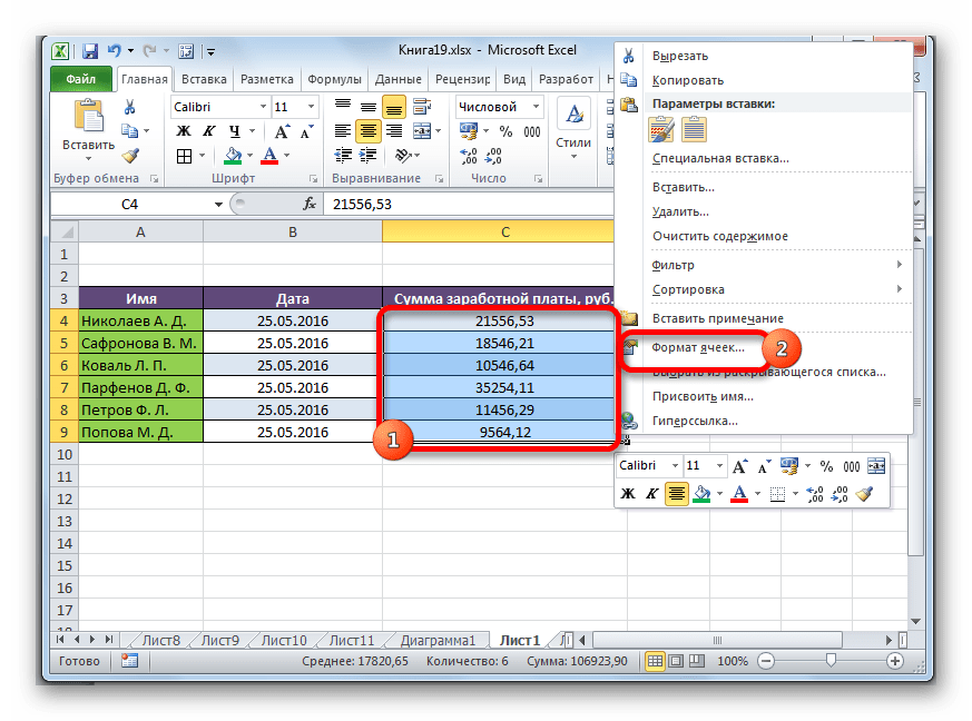
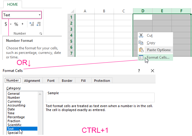
1. Производим выделение области на листе, где нужно трансформировать запятые в точки. Выполняем щелчок правой кнопкой мышки. В запустившемся контекстном меню отмечаем пункт «Формат ячеек…». Те пользователи, которые предпочитают пользоваться альтернативными вариантами с применением «горячих клавиш», после выделения могут набрать комбинацию клавиш Ctrl+1.



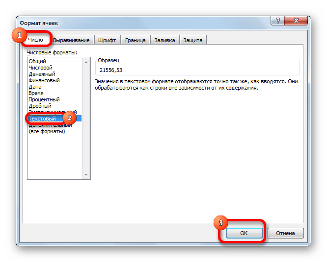
2. Производится запуск окна форматирования. Производим передвижение во вкладку «Число». В группе параметров «Числовые форматы» перемещаем выделение в позицию «Текстовый». Для того чтобы сохранить внесенные изменения, щелкаем по кнопке «OK». Формат данных в выбранном диапазоне будет преобразован в текстовый.



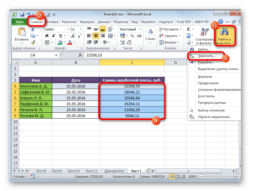
3. Опять выделяем целевой диапазон. Это важный нюанс, ведь без предварительного выделения трансформация будет произведена по всей области листа, а это далеко не всегда нужно. После того, как область выделена, передвигаемся во вкладку «Главная». Щелкаем по кнопке «Найти и выделить», которая размещена в блоке инструментов «Редактирование» на ленте. Затем открывается небольшое меню, в котором следует выбрать пункт «Заменить…».



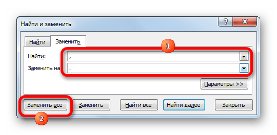
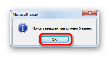
4. После этого запускается инструмент «Найти и заменить» во вкладке «Заменить». В поле «Найти» устанавливаем знак «,», а в поле «Заменить на» — «.». Щелкаем по кнопке «Заменить все».



5. Открывается информационное окно, в котором предоставляется отчет о выполненной трансформации. Делаем щелчок по кнопке «OK».

Программа выполняет процедуру трансформации запятых на точки в выделенном диапазоне. На этом данную задачу можно считать решенной. Но следует помнить, что данные, замененные таким способом будут иметь текстовый формат, а, значит, не смогут быть использованными в вычислениях.

Урок: Замена символов в Excel

Способ 2: применение функции

Второй способ предполагает применение оператора ПОДСТАВИТЬ. Для начала с помощью этой функции преобразуем данные в отдельном диапазоне, а потом скопируем их на место исходного.

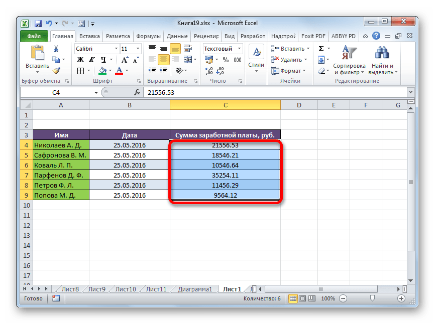
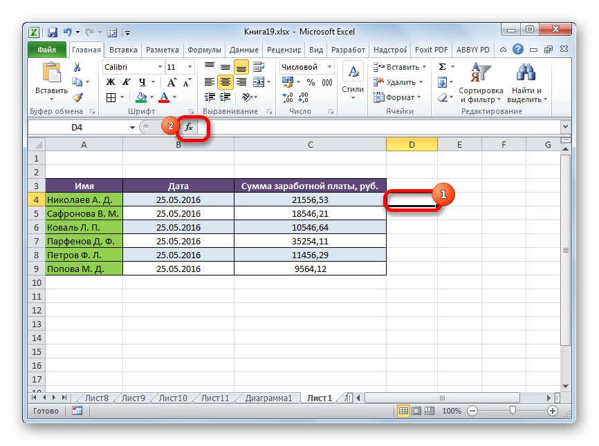
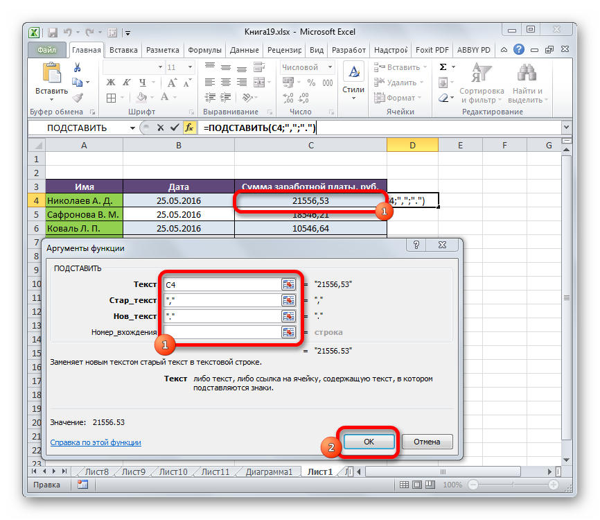
1. Выделяем пустую ячейку напротив первой ячейки диапазона с данными, в котором запятые следует трансформировать в точки. Щелкаем по пиктограмме «Вставить функцию», размещенную слева от строки формул.



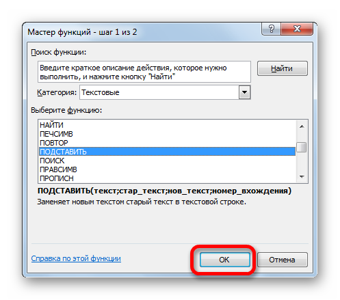
2. После этих действий будет запущен Мастер функций. Ищем в категории «Тестовые» или «Полный алфавитный перечень» наименование «ПОДСТАВИТЬ». Выделяем его и щелкаем по кнопке «OK».





3. Открывается окно аргументов функции. Она имеет три обязательных аргумента «Текст», «Старый текст» и «Новый текст». В поле «Текст» нужно указать адрес ячейки, где размещены данные, которые следует изменить. Для этого устанавливаем курсор в данное поле, а затем щелкаем мышью на листе по первой ячейке изменяемого диапазона. Сразу после этого адрес появится в окне аргументов. В поле «Старый текст» устанавливаем следующий символ – «,». В поле «Новый текст» ставим точку – «.». После того, как данные внесены, щелкаем по кнопке «OK».



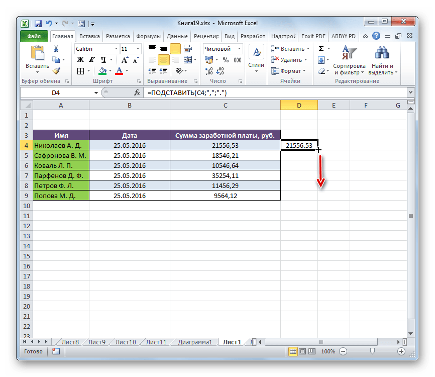
4. Как видим, для первой ячейки преобразование выполнено успешно. Подобную операцию можно провести и для всех других ячеек нужного диапазона. Хорошо, если этот диапазон небольшой. Но что делать, если он состоит из множества ячеек? Ведь на преобразование подобным образом, в таком случае, уйдет огромное количество времени. Но, процедуру можно значительно ускорить, скопировав формулу ПОДСТАВИТЬ с помощью маркера заполнения.

   Устанавливаем курсор на правый нижний край ячейки, в которой содержится функция. Появляется маркер заполнения в виде небольшого крестика. Зажимаем левую кнопку мыши и тянем этот крестик параллельно области, в которой нужно трансформировать запятые в точки.



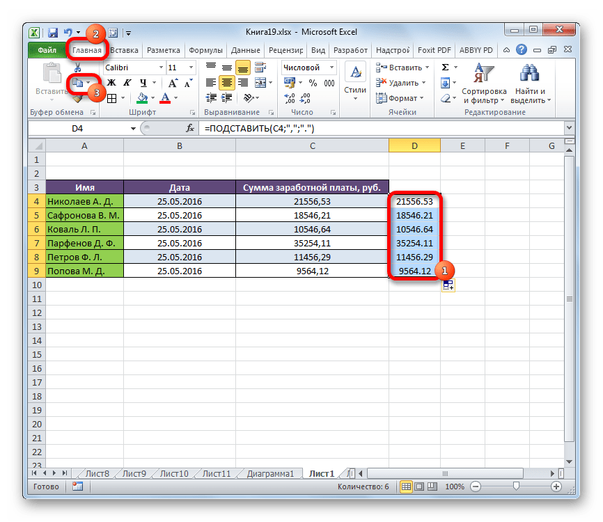
5. Как видим, все содержимое целевого диапазона было преобразовано в данные с точками вместо запятых. Теперь нужно скопировать результат и вставить в исходную область. Выделяем ячейки с формулой. Находясь во вкладке «Главная», щелкаем по кнопке на ленте «Копировать», которая расположена в группе инструментов «Буфер обмена». Можно сделать и проще, а именно после выделения диапазона набрать комбинацию клавиш на клавиатуре Ctrl+1.



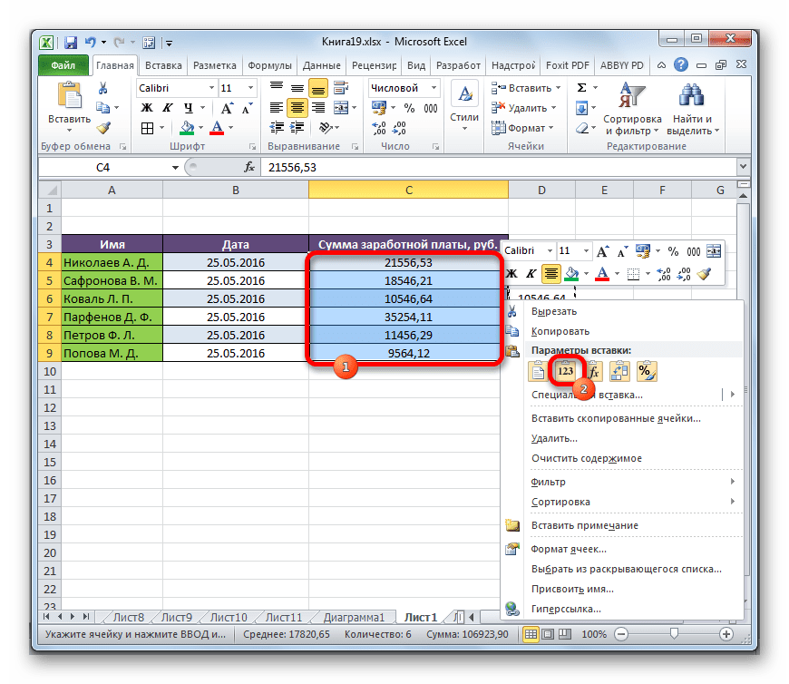
6. Выделяем исходный диапазон. Щелкаем по выделению правой кнопкой мыши. Появляется контекстное меню. В нем выполняем щелчок по пункту «Значения», который расположен в группе «Параметры вставки». Данный пункт обозначен цифрами «123».



7. После этих действий значения будут вставлены в соответствующий диапазон. При этом запятые будут трансформированы в точки. Чтобы удалить уже не нужную нам область, заполненную формулами, выделяем её и щелкаем правой кнопкой мыши. В появившемся меню выбираем пункт «Очистить содержимое».

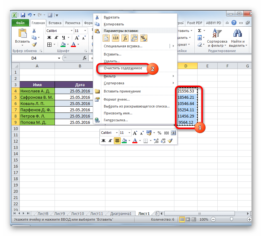
Преобразование данных по смене запятых на точки выполнено, а все ненужные элементы удалены.

Урок: Мастер функций в Excel

Способ 3: Использование макроса

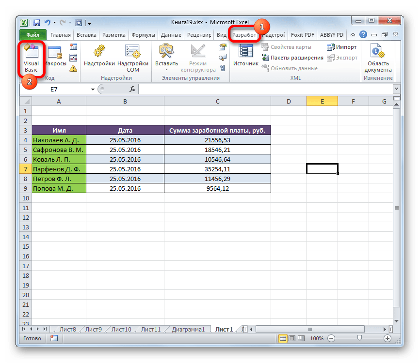
Следующий способ трансформации запятых в точки связан с использованием макросов. Но, дело состоит ещё в том, что по умолчанию макросы в Экселе отключены.

Прежде всего, следует включить макросы, а также активировать вкладку «Разработчик», если в вашей программе они до сих пор не активированы. После этого нужно произвести следующие действия:

1. Перемещаемся во вкладку «Разработчик» и щелкаем по кнопке «Visual Basic», которая размещена в блоке инструментов «Код» на ленте.



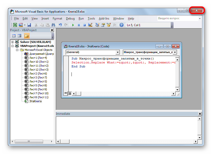
2. Открывается редактор макросов. Производим вставку в него следующего кода:

   Sub Макрос_трансформации_запятых_в_точки()
Selection.Replace What:=",", Replacement:="."
End Sub

   Завершаем работу редактора стандартным методом, нажав на кнопку закрытия в верхнем правом углу.



3. Далее выделяем диапазон, в котором следует произвести трансформацию. Щелкаем по кнопке «Макросы», которая расположена все в той же группе инструментов «Код».



4. Открывается окно со списком имеющихся в книге макросов. Выбираем тот, который недавно создали через редактор. После того, как выделили строку с его наименованием, щелкаем по кнопке «Выполнить».

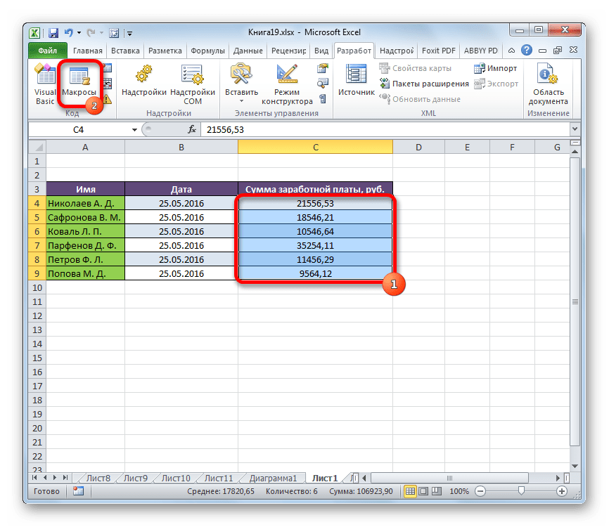
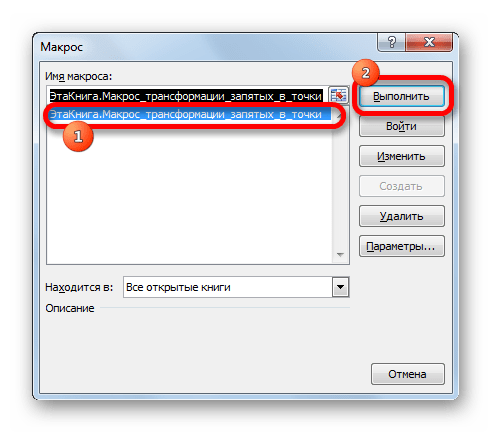
Выполняется преобразование. Запятые будут трансформированы в точки.

Урок: Как создать макрос в Excel

Способ 4: настройки Эксель

Следующий способ единственный среди вышеперечисленных, при котором при трансформации запятых в точки выражение будет восприниматься программой как число, а не как текст. Для этого нам нужно будет поменять системный разделитель в настройках с запятой на точку.

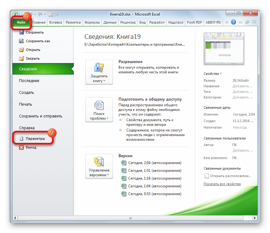
1. Находясь во вкладке «Файл», щелкаем по наименованию блока «Параметры».



2. В окне параметров передвигаемся в подраздел «Дополнительно». Производим поиск блока настроек «Параметры правки». Убираем флажок около значения «Использовать системные разделители». Затем в пункте «Разделитель целой и дробной части» производим замену с «,» на «.». Для введения параметров в действие щелкаем по кнопке «OK».

После вышеуказанных действий запятые, которые использовались в качестве разделителей для дробей, будут преобразованы в точки. Но, главное, выражения, в которых они используются, останутся числовыми, а не будут преобразованы в текстовые.

Существует ряд способов преобразования запятых в точки в документах Excel. Большинство из этих вариантов предполагают изменение формата данных с числового на текстовый. Это ведет к тому, что программа не может задействовать эти выражения в вычислениях. Но также существует способ произвести трансформацию запятых в точки с сохранением исходного форматирования. Для этого нужно будет изменить настройки самой программы.

The use of a decimal point instead of a comma can lead to significant consequences in Excel calculations. These mistakes most frequently occur when data are imported into the spreadsheet from other sources.

If a decimal point is used instead of a comma in fractions, the program automatically perceives them as a text data type. Therefore, before doing mathematical calculations and computations you should format and prepare imported data.



How to change decimal point to comma in Excel?

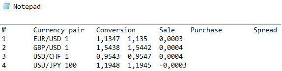
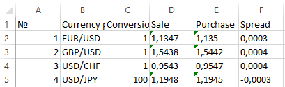
Highlight and copy data from the spreadsheet given below:

№	Currency pair	Conversion	Sale	Purchase	Spread
1	EUR/USD	1	1,1347	1,1350	0,0003
2	GBP/USD	1	1,5438	1,5442	0,0004
3	USD/CHF	1	0,9543	0,9547	0,0004
4	USD/JPY	100	1,1948	1,1945	-0,0003

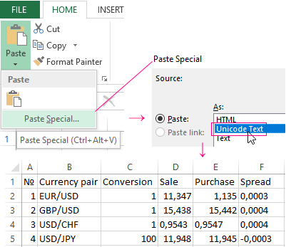
Now go to the worksheet and right-click cell A1. Select «Paste Special» option in the appeared shortcut menu. In the dialog box select «Unicode Text» and click OK.

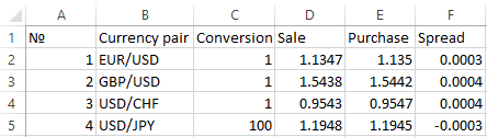
As you can see, Excel recognizes only those numbers, which are located in column C. Values in this column are right aligned. In other columns values are left aligned. In all cells the format is «General» by default.

Note. If you copy data from other sources without Paste Special, format is copied together with other data. In this case «General» format of cells (by default) can be changed, making it impossible to distinguish visually whether the number or the text has been recognized.

All further actions should be performed on a blank worksheet. Delete everything from the sheet and open a new one for further work.

To convert decimal point to comma in imported data you can use 4 methods:



Method 1: converting decimal point to comma in Excel through Notepad

Windows Notepad doesn’t require applying complicated settings or functions. It is merely an intermediary in copying and preparing data.

1. Copy the data from the original spreadsheet on this page. Open Windows Notepad («Start» — «All programs» — «Standard» — «Notepad») and paste the copied data into it for preparation.



2. Select «Replace» option in «Edit» menu (or use a combination of hot keys CTRL + H). In the appeared dialog box, type decimal point (.) in «What» field and comma (,) in «With» field. Then click «Replace All» button.

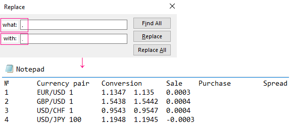
Notepad program replaced all decimal points with commas. Now the data is ready for copying and pasting in the worksheet.

This is a rather simple, but very effective way.

Method 2: temporary change of Excel settings

Before you change a decimal point to a comma in Excel, correctly evaluate the set task. Perhaps it is better to make the program temporarily perceive a point, as a decimal separator in fractional numbers. In the settings you need to specify that in fractional numbers the separator is a decimal point instead of a comma.

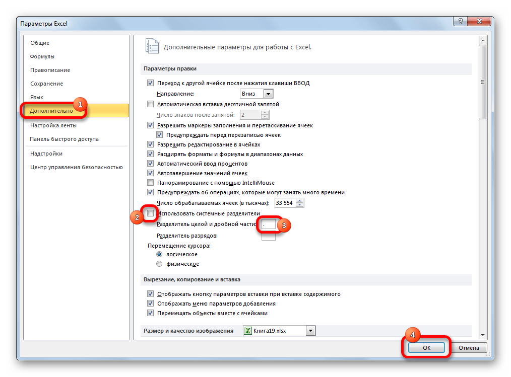
To do this, open «FILE»-«Options»-«Advanced». You should temporarily uncheck «Used system separators» in «Editing options» section. Then remove a comma and enter a decimal point in «Decimal separator и Thousands separator» field.

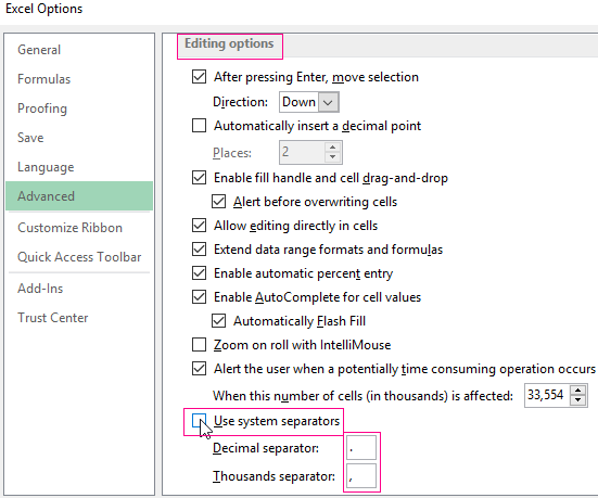
After performing the calculations, you are strongly recommended to return the default settings.

Attention! This method works if you make all the changes before importing data, not after it.

Method 3: temporary change of Windows system settings

The principle of this method is similar to the previous one. But here you change the similar settings in Windows. You need to replace the comma with a decimal point in the settings of the regional operating system standards. Now, more details on how to do this.

Open «Start» — «Control Panel» — «Languages and Regional Standards». Click on «Advanced options» button. In the appeared window, make change in the first field «Delimiter of integer and fractional part» and enter the value you need. Then click OK and OK.

Attention! If you open this file on another computer where other system parameters of regional standards are set, you may experience computational problems.

Method 4: using find and replace function in Excel

This method is similar to the first one. Only here we use the same function from Notepad, but this time in Excel itself.

Applying this method, in contrast to the above mentioned ones, first insert the copied spreadsheet on a blank worksheet, and then prepare it for computations and calculations.

An important drawback of this method is the complexity of its implementation, if some fractional numbers with a decimal point after the insertion have been recognized as a date, and not as a text. Therefore, first get rid of the dates, and then deal with the text and the decimal points.

1. Pre-select the columns where the fractional numbers with a decimal point as a separator will be located. In this case, these are three D: F columns.
2. Set the text format of cells for the selected range to avoid the automatic conversion of some numbers to the date format. To do this, select the text format from the drop-down list on «HOME» tab in «Number» section. Alternatively, press CTRL + 1, select «Number» tab in the appeared «Format Cells» window, and select «Text» in «Category:» section.



3. Copy the spreadsheet and right click on cell A1. Select «Paste Special» option in the shortcut menu. Select «Unicode text» and click OK. Note how the values in cells D2, D3, D5, E3, E2, E5, are now displayed in contrast to the very first spreadsheet copying.



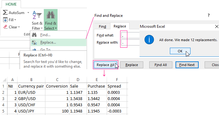
4. Click «HOME»-«Find and Select»-«Replace» tool (or press CTRL + H).



5. In the window that appears, enter a decimal point in «Find what:» field, and a comma in the second «Replace width:» field. Then click «Replace All».
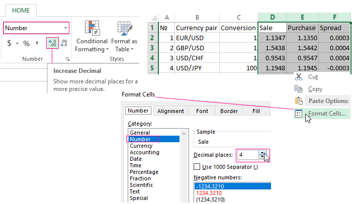
6. Select 3 columns D: F again and change the format of the cells to «Number» (or press hot keys CTRL+SHIFT+1). Don’t forget to increase decimal as described in point 4.

All decimal points have been replaced with commas. The text has automatically converted to a number.

Instead of the 4th and 5th items, you can use in a separate column a formula with the following functions:

For example, select the range of cells G2: I5, enter this formula and press CTRL + Enter. Then move the cell values of G2: I5 range to D2: F5 range.

This formula finds a decimal point in the text with the help of =FIND() function. Then the second function changes it to a comma. And =VALUE() function converts the obtained result to a number.

This seems to be a continuation to my answer to your previous question, but if so I think you misunderstood what I meant. I’ve taken your code and amended it with my suggestion, but I’ve not tested it:

Public Sub VirgulaPunct()
Dim oRow As Range
Dim cell As Range
Dim i As Long, j As Long
Dim MyString As String
Dim aux As String

    Application.ScreenUpdating = False

    For i = Selection(Selection.Count).Row To Selection.Cells(1, 1).Row Step -1

        For j = Selection(Selection.Count).Column To Selection.Cells(1, 1).Column Step -1
            MyString = Cells(i, j).Value
            MyString = Replace(MyString, ",", ";+;", 1)
            MyString = Replace(MyString, ".", ",", 1)
            MyString = Replace(MyString, ";+;", ".", 1)
            Cells(i, j).Value = MyString
        Next j
    Next i
    Application.ScreenUpdating = True
End Sub

So as I said in my previous answer, I do 3 calls to Replace, but I do them for the whole string rather than per character in the string.

For future reference, it would probably be better if you updated your original question rather than to create a new one and then you could leave a comment for me under my answer and I’d seen that you have done so.

Change Separators from Commas to Decimals or Decimals to Commas in Microsoft Excel

by Avantix Learning Team | Updated November 23, 2021

Applies to: Microsoft^® Excel^® 2013, 2016, 2019 and 365 (Windows)

Depending on your country or region, Excel may display decimal points or dots instead of commas for larger numbers. The decimal point (.) or comma (,) is used as the group separator in different regions in the world. You can change commas to decimal points or dots or vice versa in your Excel workbook temporarily or permanently. The default display of commas or decimal points is based on your global system settings (Regional Settings in the Control Panel) and Excel Options.

If you want to use a decimal point instead of a comma as a group or thousands separator, which is different from your Regional Settings, this can lead to issues with your Excel calculations.

Excel recognizes numbers without group or thousands separators so these separators are actually a format.

Your Regional Settings in your Control Panel on your device are used by default by Excel to determine if decimals should be a period or dot (used in the US and in English Canada for example) or if decimals are a comma (used in many European countries and French Canada).

Recommended article: 10 Great Excel Pivot Table Shortcuts

Do you want to learn more about Excel? Check out our virtual classroom or live classroom Excel courses >

Changing commas to decimals by changing global system settings

It’s important to enter data in Excel in accordance with your global system settings in the Control Panel. For example, if you enter the number 1045.35 and your system is set with US as the region, the period is used as the decimal separator. If you enter the number 1045,35 in France, the comma is used as the decimal separator based on system settings with France as the region.

Below is the Control Panel in Windows 10:

To change the Regional Settings in the Control Panel in Windows 10:

1. In the Start a search box on the bottom left of the screen, type Control Panel. The Control Panel appears.
2. Click Clock and Region. This may appear as Languages and Regional Standards.
3. Below Region, click Change Date, Time, or Number Formats. A dialog box appears. If you change the region, Excel (and other programs) will use settings based on the selected region so US would use periods as decimals and commas as thousands separators.
4. If you don’t want to change the region, click Additional settings. A Customize Format dialog box appears.
5. Click the Numbers tab.
6. Select the desired options in Decimal symbol and Digit grouping symbol. You can also change other options in this dialog box (such as the format of negatives).
7. Click OK twice.

Below is the Customize Format dialog box:

Keep in mind that this will change defaults on your device for all Excel workbooks (as well as other programs like Microsoft Access or Microsoft Project). If another user opens the workbook on a different device, the separators will display based on their system settings.

Changing commas to decimals and vice versa by changing Excel Options

You can also change Excel Options so that commas display as the group or thousands separator instead of decimals and vice versa. This option will affect any workbook you open after you have made this change.

To change Excel Options so that commas display as the thousands separator and decimals appear as the decimal separator (assuming your global settings in Regional Settings are set in the opposite way):

1. Click the File tab in the Ribbon.
2. Click Options.
3. In the categories on the left, click Advanced.
4. Uncheck Use system separators in the Editing area.
5. In the Decimal separator box, enter the desired character such as a decimal or period (.).
6. In the Thousands separator box, enter the desired character such as a comma (,).
7. Click OK.

Below is the Options dialog box where Use system separators has been turned off and a decimal and comma have been entered as separators:

You may want to change the Options back to Use system separators when you have finished your task.

Creating a formula to change separators and format using current system separators

Another alternative is to write a formula in another cell or column to convert separators. This works well if the data is text with separators that are not used in the current system settings. If you write a formula to convert text to numbers, you can keep the original values as well. In Excel 2013 or later, you can use the NUMBERVALUE function to convert the text to numbers.

The NUMBERVALUE function has the following arguments:

Text – The text to convert to a number.

Decimal_separator – The character used in the original cell to separate the integer and fractional part of the result.

Group_separator – The character used in the original cell to separate groupings of numbers, such as thousands from hundreds and millions from thousands.

The function is entered as follows:

=NUMBERVALUE(Text,Decimal_separator, Group_separator)

For example, if you have 2.500.300,00 in A1 and your device is set to US in the Regional Settings, you could enter the following formula in B1:

=NUMBERVALUE(A1,»,»,».»)

The value that is returned will normally appear as a number without formatting. You can then apply appropriate formatting by pressing Ctrl + 1 and using Format Cells to apply formatting with system separators.

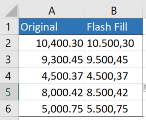
Changing separators using Flash Fill

Flash Fill is a utility that is available in Excel 2013 and later versions and can be used to clean up and / or reformat data. It is not a formula, so if the original data changes, you’ll need to rerun Flash Fill.

In the example below, the numbers entered in column A are formatted using system settings (US in this case). In column B, we have entered sample data in B2 and B3 with different separators (periods for the group separator and commas for the decimal separator). It’s usually best to enter a few examples to show Excel the pattern. You’ll need data with a pattern to the left in order to use Flash Fill. Once you have entered a few examples of the pattern in cells to the right of the original data, in the cell below the samples (in this case in cell B4) press Ctrl + E. Flash Fill will fill in the remaining cells until it reaches the end of the data set.

The following example was created using Flash Fill in column B (the data that is filled in column B is text):

For more information, check out How to Use Flash Fill in Excel (4 Ways with Shortcuts).

Changing commas to decimals in an Excel worksheet for a selected range using Replace

You can use the Replace command to replace commas with decimals or vice versa In a range of cells on a worksheet. It’s important to understand that this will change the range of cells to text so you won’t be able to use certain functions like SUM. You may want to replace on a copy of the data.

To change commas to decimals using Replace:

1. Select the range of cells in which you want to replace commas with decimals. You may select a range of cells, a column or columns or the entire worksheet.
2. Press Ctrl + 1 or right-click and select Format Cells. A dialog box appears.
3. Click the Number tab.
4. In the categories on the left, click Text and then click OK. Notably, the data will be text not numbers.
5. Click the Home tab in the Ribbon and in the Editing group, click Find & Select. A drop-down menu appears.
6. Click Replace. Alternatively, press Ctrl + H. A dialog box appears.
7. In the Find and Replace dialog box, click the Replace tab.
8. In the Find what box, enter a comma (the character that you want to find).
9. In the Replace with box, enter a decimal or period (the character that you want to replace).
10. Click Replace All if you are sure that you want to replace all symbols or characters in the selected range. Click Replace if you want to find and replace one by one in the selected range. Click Find All if you want to find all of the characters to be replaced first and then decide if you want to replace all. Click Find Next if you want to find characters one by one and decide if you want to replace each character by clicking Replace. After replacing all characters, Excel displays a dialog box with the number of replacements.

Below is the Find and Replace dialog box with a comma (,) entered in the Find what box and a decimal (.) in the Replace with box:

In the previous example, only commas were changed to decimals but you may have data that has both commas and decimals (like 1,475.55). In this case, you would need to Replace multiple times.

To change commas to decimals and decimals to commas using Replace:

1. Select the range of cells in which you want to replace commas with decimals and decimals with commas. You may select a range of cells, a column or columns or the entire worksheet.
2. Press Ctrl + 1 or right-click and select Format Cells. A dialog box appears.
3. Click the Number tab.
4. In the categories on the left, click Text and then click OK. Notably, the data will be text not numbers.
5. Click the Home tab in the Ribbon and in the Editing group, click Find & Select. A drop-down menu appears.
6. Click Replace. Alternatively, press Ctrl + H. A dialog box appears.
7. In the Find and Replace dialog box, click the Replace tab.
8. In the Find what box, enter a decimal.
9. In the Replace with box, enter an asterisk (*).
10. Click Replace All if you are sure that you want to replace all symbols or characters in the selected range. Click Replace if you want to find and replace one by one in the selected range. Click Find All if you want to find all of the characters to be replaced first and then decide if you want to replace all. Click Find Next if you want to find characters one by one and decide if you want to replace each character by clicking Replace. After replacing all characters, Excel displays a dialog box with the number of replacements.
11. In the Find what box, enter a comma.
12. In the Replace with box, enter a decimal or period.
13. Click Replace All if you are sure that you want to replace all symbols or characters in the selected range. Click Replace if you want to find and replace one by one in the selected range. Click Find All if you want to find all of the characters to be replaced first and then decide if you want to replace all. Click Find Next if you want to find characters one by one and decide if you want to replace each character by clicking Replace. After replacing all characters, Excel displays a dialog box with the number of replacements.
14. In the Find what box, enter an asterisk (*).
15. In the Replace with box, enter a comma.
16. Click Replace All if you are sure that you want to replace all symbols or characters in the selected range. Click Replace if you want to find and replace one by one in the selected range. Click Find All if you want to find all of the characters to be replaced first and then decide if you want to replace all. Click Find Next if you want to find characters one by one and decide if you want to replace each character by clicking Replace. After replacing all characters, Excel displays a dialog box with the number of replacements.

Again, the result will be text, not numbers.

Subscribe to get more articles like this one

Did you find this article helpful? If you would like to receive new articles, join our email list.

More resources

How to Convert Text to Numbers in Excel

How to Highlight Errors, Blanks and Duplicates in Excel Worksheets

3 Excel Strikethrough Shortcuts to Cross Out Text or Values in Cells

How to Replace Blank Cells in Excel with Zeros (0), Dashes (-) or Other Values

Use Conditional Formatting in Excel to Highlight Dates Before Today (3 Ways)

Related courses

Microsoft Excel: Intermediate / Advanced

Microsoft Excel: Data Analysis with Functions, Dashboards and What-If Analysis Tools

Microsoft Excel: Introduction to Power Query to Get and Transform Data

Microsoft Excel: New and Essential Features and Functions in Excel 365

Microsoft Excel: Introduction to Visual Basic for Applications (VBA)

VIEW MORE COURSES >

Our instructor-led courses are delivered in virtual classroom format or at our downtown Toronto location at 18 King Street East, Suite 1400, Toronto, Ontario, Canada (some in-person classroom courses may also be delivered at an alternate downtown Toronto location). Contact us at info@avantixlearning.ca if you’d like to arrange custom instructor-led virtual classroom or onsite training on a date that’s convenient for you.

Copyright 2023 Avantix^® Learning

Microsoft, the Microsoft logo, Microsoft Office and related Microsoft applications and logos are registered trademarks of Microsoft Corporation in Canada, US and other countries. All other trademarks are the property of the registered owners.

Avantix Learning |18 King Street East, Suite 1400, Toronto, Ontario, Canada M5C 1C4 | Contact us at info@avantixlearning.ca