Excel replace function all

REPLACE, REPLACEB functions

This article describes the formula syntax and usage of the REPLACE and REPLACEB function in Microsoft Excel.

Description

REPLACE replaces part of a text string, based on the number of characters you specify, with a different text string.

REPLACEB replaces part of a text string, based on the number of bytes you specify, with a different text string.

These functions may not be available in all languages.

REPLACE is intended for use with languages that use the single-byte character set (SBCS), whereas REPLACEB is intended for use with languages that use the double-byte character set (DBCS). The default language setting on your computer affects the return value in the following way:

REPLACE always counts each character, whether single-byte or double-byte, as 1, no matter what the default language setting is.

REPLACEB counts each double-byte character as 2 when you have enabled the editing of a language that supports DBCS and then set it as the default language. Otherwise, REPLACEB counts each character as 1.

The languages that support DBCS include Japanese, Chinese (Simplified), Chinese (Traditional), and Korean.

Syntax

REPLACE(old_text, start_num, num_chars, new_text)

REPLACEB(old_text, start_num, num_bytes, new_text)

The REPLACE and REPLACEB function syntax has the following arguments:

Old_text Required. Text in which you want to replace some characters.

Start_num Required. The position of the character in old_text that you want to replace with new_text.

Num_chars Required. The number of characters in old_text that you want REPLACE to replace with new_text.

Num_bytes Required. The number of bytes in old_text that you want REPLACEB to replace with new_text.

New_text Required. The text that will replace characters in old_text.

Example

Copy the example data in the following table, and paste it in cell A1 of a new Excel worksheet. For formulas to show results, select them, press F2, and then press Enter. If you need to, you can adjust the column widths to see all the data.

Источник

REPLACE Function

Summary

The Excel REPLACE function replaces characters specified by location in a given text string with another text string. For example =REPLACE(«XYZ123″,4,3,»456») returns «XYZ456».

Purpose

Return value

Arguments

• old_text — The text to replace.
• start_num — The starting location in the text to search.
• num_chars — The number of characters to replace.
• new_text — The text to replace old_text with.

Syntax

Usage notes

The REPLACE function replaces characters in a text string by position. The REPLACE function is useful when the location of the text to be replaced is known or can be easily determined.

REPLACE function takes four separate arguments. The first argument, old_text, is the text string to be processed. The second argument, start_num is the numeric position of the text to replace. The third argument, num_chars, is the number of characters that should be replaced. The last argument, new_text, is the text to use for the replacement.

Examples

To replace the «C» in the path below with a «D»:

To replace 3 characters starting at the 4th character:

You can use REPLACE to remove text by specifying an empty string («») for new_text. The formula below uses REPLACE to remove the first character from the string «XYZ»:

The example below removes the first 4 characters:

Use the REPLACE function to replace text at a known location in a text string. Use the SUBSTITUTE function to replace text by searching when the location is not known. Use FIND or SEARCH to determine the location of specific text.

Источник

Find or replace text and numbers on a worksheet

Use the Find and Replace features in Excel to search for something in your workbook, such as a particular number or text string. You can either locate the search item for reference, or you can replace it with something else. You can include wildcard characters such as question marks, tildes, and asterisks, or numbers in your search terms. You can search by rows and columns, search within comments or values, and search within worksheets or entire workbooks.

Tip: You can also use formulas to replace text. Check out the SUBSTITUTE function or REPLACE, REPLACEB functions to learn more.

To find something, press Ctrl+F, or go to Home > Editing > Find & Select > Find.

Note: In the following example, we’ve clicked the Options >> button to show the entire Find dialog. By default, it will display with Options hidden.

In the Find what: box, type the text or numbers you want to find, or click the arrow in the Find what: box, and then select a recent search item from the list.

Tips: You can use wildcard characters — question mark ( ?), asterisk ( *), tilde (

) — in your search criteria.

Use the question mark (?) to find any single character — for example, s?t finds «sat» and «set».

Use the asterisk (*) to find any number of characters — for example, s*d finds «sad» and «started».

) followed by ?, *, or

to find question marks, asterisks, or other tilde characters — for example, fy91

Click Find All or Find Next to run your search.

Tip: When you click Find All, every occurrence of the criteria that you are searching for will be listed, and clicking a specific occurrence in the list will select its cell. You can sort the results of a Find All search by clicking a column heading.

Click Options>> to further define your search if needed:

Within: To search for data in a worksheet or in an entire workbook, select Sheet or Workbook.

Search: You can choose to search either By Rows (default), or By Columns.

Look in: To search for data with specific details, in the box, click Formulas, Values, Notes, or Comments.

Note: Formulas, Values, Notes and Comments are only available on the Find tab; only Formulas are available on the Replace tab.

Match case — Check this if you want to search for case-sensitive data.

Match entire cell contents — Check this if you want to search for cells that contain just the characters that you typed in the Find what: box.

If you want to search for text or numbers with specific formatting, click Format, and then make your selections in the Find Format dialog box.

Tip: If you want to find cells that just match a specific format, you can delete any criteria in the Find what box, and then select a specific cell format as an example. Click the arrow next to Format, click Choose Format From Cell, and then click the cell that has the formatting that you want to search for.

Replace

To replace text or numbers, press Ctrl+H, or go to Home > Editing > Find & Select > Replace.

Note: In the following example, we’ve clicked the Options >> button to show the entire Find dialog. By default, it will display with Options hidden.

In the Find what: box, type the text or numbers you want to find, or click the arrow in the Find what: box, and then select a recent search item from the list.

Tips: You can use wildcard characters — question mark ( ?), asterisk ( *), tilde (

) — in your search criteria.

Use the question mark (?) to find any single character — for example, s?t finds «sat» and «set».

Use the asterisk (*) to find any number of characters — for example, s*d finds «sad» and «started».

) followed by ?, *, or

to find question marks, asterisks, or other tilde characters — for example, fy91

In the Replace with: box, enter the text or numbers you want to use to replace the search text.

Click Replace All or Replace.

Tip: When you click Replace All, every occurrence of the criteria that you are searching for will be replaced, while Replace will update one occurrence at a time.

Click Options>> to further define your search if needed:

Within: To search for data in a worksheet or in an entire workbook, select Sheet or Workbook.

Search: You can choose to search either By Rows (default), or By Columns.

Look in: To search for data with specific details, in the box, click Formulas, Values, Notes, or Comments.

Note: Formulas, Values, Notes and Comments are only available on the Find tab; only Formulas are available on the Replace tab.

Match case — Check this if you want to search for case-sensitive data.

Match entire cell contents — Check this if you want to search for cells that contain just the characters that you typed in the Find what: box.

If you want to search for text or numbers with specific formatting, click Format, and then make your selections in the Find Format dialog box.

Tip: If you want to find cells that just match a specific format, you can delete any criteria in the Find what box, and then select a specific cell format as an example. Click the arrow next to Format, click Choose Format From Cell, and then click the cell that has the formatting that you want to search for.

There are two distinct methods for finding or replacing text or numbers on the Mac. The first is to use the Find & Replace dialog. The second is to use the Search bar in the ribbon.

Источник

Excel Replace Function

The Excel Replace function is similar to the Excel Substitute Function. The difference between the two functions is:

• The Replace function replaces text in a specified position of a supplied string;
• The Substitute function replaces one or more instances of a given text string.

Function Description

The Excel Replace function replaces all or part of a text string with another string.

The syntax of the function is:

Where the function arguments are:

old_text	—	The original text string, that you want to replace a part of.
start_num	—	The position, within old_text , of the first character that you want to replace.
num_chars	—	The number of characters to replace.
new_text	—	The replacement text.

Note that the Excel Replace Function is not suitable for languages that use the double-byte character set (e.g. Chinese, Japanese, Korean). These languages should use the ReplaceB function, which is explained on the Microsoft Office website.

Replace Function Examples

Column B of the following spreadsheet shows two examples of the Excel Replace Function.

A	B
1	test string	=REPLACE( A1, 7, 3, «X» )
2	second test string	=REPLACE( A2, 8, 4, «XXX» )

A	B
1	test string	test sXng
2	second test string	second XXX string

For further information and examples of the Excel Replace function, see the Microsoft Office website.

Replace Function Error

If you get an error from the Excel Replace function, this is likely to be the #VALUE! error:

Occurs if either:

• The supplied start_num argument is negative or is a non-numeric value

or

• The supplied num_chars argument is negative or is non-numeric.

Common Problem — Use of the Excel Replace Function with Numbers, Dates and Times

The Excel Replace function is designed for use with text strings and returns a text string. Therefore, if you attempt to use the replace function with a date, time or a number, you may get unexpected results.

If you are not planning to use the date, time or number in further calculations, you could solve this problem by converting these values into text, using the Excel Text To Columns tool. To do this:

Use the mouse to select the cell(s) you want to convert to text (this must not span more than one column);

The Replace function should now work as expected on the values that have been converted to text.

Источник

Examples of working with text function REPLACE in Excel

REPLACE function is included in the text functions of MS Excel and is intended to replace a specific area of the text string containing the source text on the specified text line (new text).

How does the REPLACE function in Excel work?

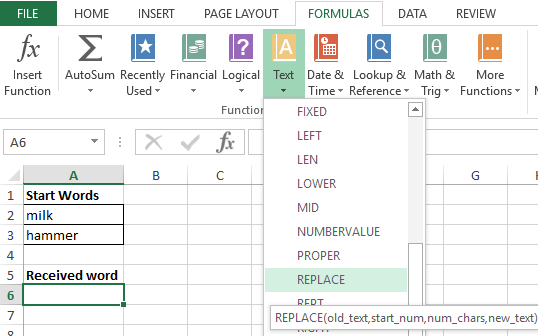
Example 1. In order to study in detail the operation of this function, we consider one of the simplest examples. Suppose we have several words in different columns, we need to get new words using the original ones. For this example, in addition to our main function REPLACE, we also use the RIGHT function — this function serves to return a certain number of characters from the end of a line of text. That is, for example, we have two words: milk and a skating rink, as a result we must get the word hammer.

REPLACE function in Excel and examples of its use

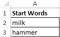
1. Create a table with words on the sheet of the Excel spreadsheet workbook, as shown in the figure:
2. Next, on the sheet of the workbook, we will prepare an area for placing our result — the resulting word “hammer”, as shown below. Place the cursor in cell A6 and call the function REPLACE:
3. Fill the function with the arguments shown in the figure:

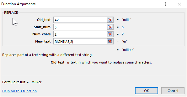
Let us explain the choice of these parameters as follows: cell A2 was chosen as the beginning of the text, the number 5 was set as beginning_, since it is from the fifth position of the word “Milk” we don’t take characters for our final word, the number_ of signs was set equal to 2, since this number It is not taken into account in the new word, as the new text, the set option RIGHT with the parameters of the cell A3 and taking the last two characters «ok».

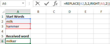
Next, click on the «OK» button and get the result:

How to REPLACE a piece of text in Excel cell?

Example 2. Consider another small example. Suppose we have columns of words in the cells of the Excel spreadsheet. It is necessary to replace their letters in certain places so as to convert them.

1. Let’s create a tablet with words on the sheet of an Excel workbook, as shown in the figure:
2. Further, on the same sheet of the working book we will prepare an area for placing our result — modified words. Fill the cells with two types of formulas as shown in the picture:

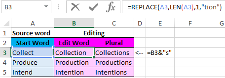
Note! In the second formula, we use the operator “&” to add the character «s» to the male surname to convert it to the female. To solve this problem, one could use the function =CONCATENATE(B3,»s») instead of the formula =B3&»s» — the result is identical. But today it is strongly recommended to abandon this formula as it has its limitations and is more demanding on resources in comparison with a simple and convenient ampersand operator.

Источник

Функция ЗАМЕНИТЬ (REPLACE) в Excel используется для замены части текста одной строки, другим текстом.

Что возвращает функция

Возвращает текстовую строку, в которой часть текста заменена на другой текст.

Синтаксис

=REPLACE(old_text, start_num, num_chars, new_text) — английская версия

=ЗАМЕНИТЬ(стар_текст;начальная_позиция;число_знаков;нов_текст) — русская версия

Аргументы функции

• old_text (стар_текст) — который вы хотите заменить;
• start_num (начальная_позиция) — стартовая позиция (порядковый номер символа), с которой вы хотите осуществить замену текста;
• num_chars (число_знаков) — количество символов, которое вы хотите заменить;
• new_text (нов_текст) — новый текст, которым вы замените текст из аргумента old_text (стар_текст).

Дополнительная информация

Аргументы стартовой позиции и количество символов для замены текста не могут быть отрицательными.

Примеры использования функции ЗАМЕНИТЬ в Excel