Excel replace all cells with text

Use the Find and Replace features in Excel to search for something in your workbook, such as a particular number or text string. You can either locate the search item for reference, or you can replace it with something else. You can include wildcard characters such as question marks, tildes, and asterisks, or numbers in your search terms. You can search by rows and columns, search within comments or values, and search within worksheets or entire workbooks.

Find

To find something, press Ctrl+F, or go to Home > Editing > Find & Select > Find.

Note: In the following example, we’ve clicked the Options >> button to show the entire Find dialog. By default, it will display with Options hidden.

In the Find what: box, type the text or numbers you want to find, or click the arrow in the Find what: box, and then select a recent search item from the list.
Tips: You can use wildcard characters — question mark (?), asterisk (*), tilde (~) — in your search criteria.
- Use the question mark (?) to find any single character — for example, s?t finds «sat» and «set».
- Use the asterisk (*) to find any number of characters — for example, s*d finds «sad» and «started».
- Use the tilde (~) followed by ?, *, or ~ to find question marks, asterisks, or other tilde characters — for example, fy91~? finds «fy91?».
Click Find All or Find Next to run your search.

Tip: When you click Find All, every occurrence of the criteria that you are searching for will be listed, and clicking a specific occurrence in the list will select its cell. You can sort the results of a Find All search by clicking a column heading.
Click Options>> to further define your search if needed:
- Within: To search for data in a worksheet or in an entire workbook, select Sheet or Workbook.
- Search: You can choose to search either By Rows (default), or By Columns.
- Look in: To search for data with specific details, in the box, click Formulas, Values, Notes, or Comments.
  
  Note: Formulas, Values, Notes and Comments are only available on the Find tab; only Formulas are available on the Replace tab.
- Match case — Check this if you want to search for case-sensitive data.
- Match entire cell contents — Check this if you want to search for cells that contain just the characters that you typed in the Find what: box.
If you want to search for text or numbers with specific formatting, click Format, and then make your selections in the Find Format dialog box.

Tip: If you want to find cells that just match a specific format, you can delete any criteria in the Find what box, and then select a specific cell format as an example. Click the arrow next to Format, click Choose Format From Cell, and then click the cell that has the formatting that you want to search for.

Replace

To replace text or numbers, press Ctrl+H, or go to Home > Editing > Find & Select > Replace.

Note: In the following example, we’ve clicked the Options >> button to show the entire Find dialog. By default, it will display with Options hidden.

In the Find what: box, type the text or numbers you want to find, or click the arrow in the Find what: box, and then select a recent search item from the list.
Tips: You can use wildcard characters — question mark (?), asterisk (*), tilde (~) — in your search criteria.
- Use the question mark (?) to find any single character — for example, s?t finds «sat» and «set».
- Use the asterisk (*) to find any number of characters — for example, s*d finds «sad» and «started».
- Use the tilde (~) followed by ?, *, or ~ to find question marks, asterisks, or other tilde characters — for example, fy91~? finds «fy91?».
In the Replace with: box, enter the text or numbers you want to use to replace the search text.
Click Replace All or Replace.

Tip: When you click Replace All, every occurrence of the criteria that you are searching for will be replaced, while Replace will update one occurrence at a time.
Click Options>> to further define your search if needed:
- Within: To search for data in a worksheet or in an entire workbook, select Sheet or Workbook.
- Search: You can choose to search either By Rows (default), or By Columns.
- Look in: To search for data with specific details, in the box, click Formulas, Values, Notes, or Comments.
  
  Note: Formulas, Values, Notes and Comments are only available on the Find tab; only Formulas are available on the Replace tab.
- Match case — Check this if you want to search for case-sensitive data.
- Match entire cell contents — Check this if you want to search for cells that contain just the characters that you typed in the Find what: box.
If you want to search for text or numbers with specific formatting, click Format, and then make your selections in the Find Format dialog box.

Tip: If you want to find cells that just match a specific format, you can delete any criteria in the Find what box, and then select a specific cell format as an example. Click the arrow next to Format, click Choose Format From Cell, and then click the cell that has the formatting that you want to search for.

There are two distinct methods for finding or replacing text or numbers on the Mac. The first is to use the Find & Replace dialog. The second is to use the Search bar in the ribbon.

Find & Replace dialog

Search bar and options

Press Ctrl+F or go to Home > Find & Select > Find.
In Find what: type the text or numbers you want to find.
Select Find Next to run your search.
You can further define your search:
- Within: To search for data in a worksheet or in an entire workbook, select Sheet or Workbook.
- Search: You can choose to search either By Rows (default), or By Columns.
- Look in: To search for data with specific details, in the box, click Formulas, Values, Notes, or Comments.
- Match case — Check this if you want to search for case-sensitive data.
- Match entire cell contents — Check this if you want to search for cells that contain just the characters that you typed in the Find what: box.

Tips: You can use wildcard characters — question mark (?), asterisk (*), tilde (~) — in your search criteria.

Use the question mark (?) to find any single character — for example, s?t finds «sat» and «set».
Use the asterisk (*) to find any number of characters — for example, s*d finds «sad» and «started».
Use the tilde (~) followed by ?, *, or ~ to find question marks, asterisks, or other tilde characters — for example, fy91~? finds «fy91?».

Press Ctrl+F or go to Home > Find & Select > Find.
In Find what: type the text or numbers you want to find.
Select Find All to run your search for all occurrences.

Note: The dialog box expands to show a list of all the cells that contain the search term, and the total number of cells in which it appears.
Select any item in the list to highlight the corresponding cell in your worksheet.

Note: You can edit the contents of the highlighted cell.

Press Ctrl+H or go to Home > Find & Select > Replace.
In Find what, type the text or numbers you want to find.
You can further define your search:
- Within: To search for data in a worksheet or in an entire workbook, select Sheet or Workbook.
- Search: You can choose to search either By Rows (default), or By Columns.
- Match case — Check this if you want to search for case-sensitive data.
- Match entire cell contents — Check this if you want to search for cells that contain just the characters that you typed in the Find what: box.
  Tips: You can use wildcard characters — question mark (?), asterisk (*), tilde (~) — in your search criteria.
  - Use the question mark (?) to find any single character — for example, s?t finds «sat» and «set».
  - Use the asterisk (*) to find any number of characters — for example, s*d finds «sad» and «started».
  - Use the tilde (~) followed by ?, *, or ~ to find question marks, asterisks, or other tilde characters — for example, fy91~? finds «fy91?».
In the Replace with box, enter the text or numbers you want to use to replace the search text.
Select Replace or Replace All.
Tips:
- When you select Replace All, every occurrence of the criteria that you are searching for is replaced.
- When you select Replace, you can replace one instance at a time by selecting Next to highlight the next instance.

Select any cell to search the entire sheet or select a specific range of cells to search.
Press Command + F or select the magnifying glass to expand the Search bar and type the text or number you want to find in the search field.
Tips: You can use wildcard characters — question mark (?), asterisk (*), tilde (~) — in your search criteria.
- Use the question mark (?) to find any single character — for example, s?t finds «sat» and «set».
- Use the asterisk (*) to find any number of characters — for example, s*d finds «sad» and «started».
- Use the tilde (~) followed by ?, *, or ~ to find question marks, asterisks, or other tilde characters — for example, fy91~? finds «fy91?».
Press return.
Notes:
- To find the next instance of the item you are searching for, press return again or use the Find dialog box and select Find Next.
- To specify additional search options, select the magnifying glass and select Search in Sheet or Search in Workbook. You can also select the Advanced option, which launches the Find dialog.
Tip: You can cancel a search in progress by pressing ESC.

Find

To find something, press Ctrl+F, or go to Home > Editing > Find & Select > Find.

Note: In the following example, we’ve clicked > Search Options to show the entire Find dialog. By default, it will display with Search Options hidden.

In the Find what: box, type the text or numbers you want to find.
Tips: You can use wildcard characters — question mark (?), asterisk (*), tilde (~) — in your search criteria.
- Use the question mark (?) to find any single character — for example, s?t finds «sat» and «set».
- Use the asterisk (*) to find any number of characters — for example, s*d finds «sad» and «started».
- Use the tilde (~) followed by ?, *, or ~ to find question marks, asterisks, or other tilde characters — for example, fy91~? finds «fy91?».
Click Find Next or Find All to run your search.

Tip: When you click Find All, every occurrence of the criteria that you are searching for will be listed, and clicking a specific occurrence in the list will select its cell. You can sort the results of a Find All search by clicking a column heading.
Click > Search Options to further define your search if needed:
- Within: To search for data within a certain selection, choose Selection. To search for data in a worksheet or in an entire workbook, select Sheet or Workbook.
- Direction: You can choose to search either Down (default), or Up.
- Match case — Check this if you want to search for case-sensitive data.
- Match entire cell contents — Check this if you want to search for cells that contain just the characters that you typed in the Find what box.

Replace

To replace text or numbers, press Ctrl+H, or go to Home > Editing > Find & Select > Replace.

Note: In the following example, we’ve clicked > Search Options to show the entire Find dialog. By default, it will display with Search Options hidden.

In the Find what: box, type the text or numbers you want to find.
Tips: You can use wildcard characters — question mark (?), asterisk (*), tilde (~) — in your search criteria.
- Use the question mark (?) to find any single character — for example, s?t finds «sat» and «set».
- Use the asterisk (*) to find any number of characters — for example, s*d finds «sad» and «started».
- Use the tilde (~) followed by ?, *, or ~ to find question marks, asterisks, or other tilde characters — for example, fy91~? finds «fy91?».
In the Replace with: box, enter the text or numbers you want to use to replace the search text.
Click Replace or Replace All.

Tip: When you click Replace All, every occurrence of the criteria that you are searching for will be replaced, while Replace will update one occurrence at a time.
Click > Search Options to further define your search if needed:
- Within: To search for data within a certain selection, choose Selection. To search for data in a worksheet or in an entire workbook, select Sheet or Workbook.
- Direction: You can choose to search either Down (default), or Up.
- Match case — Check this if you want to search for case-sensitive data.
- Match entire cell contents — Check this if you want to search for cells that contain just the characters that you typed in the Find what box.

Need more help?

You can always ask an expert in the Excel Tech Community or get support in the Answers community.

Replacing characters in text with the REPLACE function

The REPLACE function substitutes a text string with another text string.

Let’s say your boss tells you that the product IDs for a product line must be changed.

But only a part of the product ID should be changed – not all of it.

Here, the “29FA” part of all the product IDs needs to be changed to “39LU”.

To do that with the REPLACE function, we’ll walk through the syntax of the REPLACE function, which goes like this:

=REPLACE(old_text, start_num, num_chars, new_text)

Don’t worry, it’s not as daunting as it looks. It’s actually pretty straightforward👍

Step 1: Old text

The old text argument is a reference to the cell where you want to replace some text. Write:

=REPLACE(A2

Excel replace function - reference to old text argument of syntax

And put a comma to wrap up the first argument, and let’s move on to the next.

Step 2: Start num

The start_num argument determines where the REPLACE function should start replacing characters from.

In our case, the “29FA” part starts on the 3rd character in the text.

Excel replace function to replace text from a specified position

So, write:

=REPLACE(A2, 3,

Now, we’ve established where the REPLACE function should start to replace text.

Still with me? Then let’s dive into the next argument of the REPLACE syntax🤿

Step 3: Num chars

Also called the “number of characters” argument, this determines how many characters should be replaced with the new text.

Typically, this should be the length of the text you want to replace the old text with.

So, it ties together with the next argument.

If you want to replace “29FA” with “39LU”, then you’re replacing the next 4 characters.

Write:

=REPLACE(A2, 3, 4

Excel replace function - number of characters to replace

And wrap it up with a comma🎁

There are situations where this num_chars argument should be a different length than the new_text argument. I’ll tell you more about that later.

Kasper Langmann, Microsoft Office Specialist

Step 4: New text

The new_text argument is the replacement text for the old text.

So, simply write the new characters that should replace the old 4 characters:

=REPLACE(A2, 3, 4, “39LU”

Excel replace function - new text argument

Remember the double quotes when the replacement text is letters or a combination of numbers and letters.

Wrap up the formula with an end parenthesis and press Enter.

Now, the “29FA” part of the old product ID is replaced with “39LU”.

PRO TIP: Length of num_chars vs new_text

If you need the replacement text to be shorter or longer than the text it’s replacing, you can have a different length in the 3rd and 4th argument of REPLACE. Let me give you a few formula examples of that:

If you wanted to replace the “29FA” with “39L” instead, you’d write:

=REPLACE(A2, 3, 4, “39L”)

But the length of the 4th argument would be shorter than the 4 characters defined in the 3rd argument.

On the other hand, if you wanted to replace “FA” with “LLUU”, you’d write this:

=REPLACE(A2, 5, 2, “LLUU”)

Formula example Different length in number of characters and new text

Replacing text strings with the SUBSTITUTE function

If the string you want to replace doesn’t always appear in the same place, you’re better off using the SUBSTITUTE function.

The syntax of SUBSTITUTE goes like this:

=SUBSTITUTE(text, old_text, new_text, [instance_num])

This is a little different from the last syntax of the REPLACE function, so be careful not to get them mixed up⚠️

Step 1: Text

The text argument is just a cell reference to the cell where you want to replace text.

Write:

=SUBSTITUTE(A2

Excel substitute function to replace text - text argument

And of course, put a comma to go to the next argument.

Step 2: Old text

The SUBSTITUTE function doesn’t replace characters from a fixed position in a cell.

Instead, it cleverly searches for a text string and begins replacing characters from there🔍

So, if you want to replace the “FA” part of the product ID with “LU”, write:

=SUBSTITUTE(A2, “FU”

Excel substitute function - old text argument

Step 3: New text

The new_text argument is what the old text should be replaced with.

For this example, that’s “LU”.

=SUBSTITUTE(A2, “FA”, “LU”

Excel replace text - old text and new text

The new text doesn’t have to be the same length as the old text.

Kasper Langmann, Microsoft Office Specialist

Step 4: Instance num

The optional instance num argument decides how many times the text should be replaced.

This is relevant if there is more than one instance of the old text.

The instance_num argument is optional. If you leave it blank, every instance of the old text is replaced by the new text😊

In the following formula example, the first 2 product IDs each have 2 instances of the “FA”. So, the instance num argument determines whether only the first instance of “FA” is replaced with “LU” or both instances of “FA” is replaced with “LU”.

As you can see from the picture below, write 1 if you want only the first instance of “FA” to be replaced.

=SUBSTITUTE(A2, “FA”, “LU”, 1)

Or don’t use the instance num argument if every instance of “FA” should be replaced:

=SUBSTITUTE(A2, “FA”, “LU”)

Excel substitute formula examples with instance number argument for multiple replacements

And that’s how to replace text dynamically based on the location of the text you want to replace.

The difference between REPLACE and SUBSTITUTE

There are a few subtle differences between these two “replace functions”.

Both of them replace one or more characters in a text string with another text string.

The difference lies in how the first string is identified.

REPLACE selects the first string based on the position. So you might replace four characters, starting with the sixth character in the string.

SUBSTITUTE selects based on whether the string matches a predefined search. You might tell Excel to replace any instance of “FA” with “LU” for example.

Other than that, the two functions are identical👬🏻

Replace text using Find and Replace

Another way to replace text is with the ‘Find and Replace’ feature of Excel.

It’s a way to substitute characters in the original cell instead of having to add additional columns with formulas.

1. Select all the cells that contain the text to replace.

2. From the ‘Home’ tab, click ‘ Find and Select’.

3. From the Find and Replace dialog box (in the replace tab) write the text you want to replace, in the ‘Find what:’ field.

4. Still within the ‘Find and Replace’ dialog box, write the new text to replace the old text with in the ‘Replace with:’ field.

Replace text by using the find what and replace with fields from Find and Replace dialog box

5. When you click the ‘Replace all’ button, Excel replaces all instances of the old text with the new text, in the selected cells.

If you instead want to replace all instances of the text within the entire workbook, just select a single cell before opening the ‘Find and Replace’ dialog box.

(Instead of selecting multiple cells).

Kasper Langmann, Microsoft Office Specialist

That’s it – Now what?

With the REPLACE and SUBSTITUTE functions, you can replace very specific strings with other strings. You can use letters, numbers, or other characters.

In short, you can replace text with extreme accuracy. And that saves you a great deal of time when you need to make a lot of edits.

Additionally, you can use the Find and Replace tool, which is the most underrated feature of Excel.

But no one got a job offer just based on their skills to replace characters in a text in Microsoft Excel.

Luckily, there are other areas of Excel that are magnets for job offers🧲

Click here to learn IF, SUMIF, VLOOKUP, and pivot tables (yup, that’s the magnets) for FREE in my 30-minute online Excel course.

Other resources

Replacing text is often used to clean up data so it’s ready for analysis, formulas, pivot tables, etc.

Other ways of cleaning up data are with other important Excel functions like LEFT, RIGHT, MID, and LEN.

Or with one of the two ways of deleting blank rows (one better than the other). Read all about it here.

Kasper Langmann2023-01-19T12:24:59+00:00

Page load link

Источник

Is it possible to select all the bank cells in an excel sheet and put the same value in all the cells?

I just want to populate them with «null»

I have Excel student 2010

asked Dec 22, 2011 at 8:33

To put the same text in a certain number of cells do the following:

Highlight the cells you want to put text into
Type into the cell you’re currently in the data you want to be repeated
Hold Crtl and press ‘return’

You will find that all the highlighted cells now have the same data in them.
Have a nice day.

Sirko

71.8k19 gold badges147 silver badges181 bronze badges

answered May 3, 2013 at 14:50

PhoenixPhoenix

4,30410 gold badges39 silver badges53 bronze badges

OK, what you can try is

Cntrl+H (Find and Replace), leave Find What blank and change Replace With to NULL.

That should replace all blank cells in the USED range with NULL

answered Dec 22, 2011 at 11:12

Adriaan StanderAdriaan Stander

161k30 gold badges285 silver badges283 bronze badges

Here’s a tricky way to do this — select the cells that you want to replace and in Excel 2010 select F5 to bring up the «goto» box. Hit the «special» button. Select «blanks» — this should select all the cells that are blank. Enter NULL or whatever you want in the formula box and hit ctrl + enter to apply to all selected cells. Easy!

answered Jul 19, 2012 at 17:28

RobinRobin

1111 silver badge2 bronze badges

If all the cells are under one column, you could just filter the column and then select «(blank)» and then insert any value into the cells. But be careful, press «alt + 4» to make sure you are inserting value into the visible cells only.

answered Sep 30, 2014 at 15:26

user2722393user2722393

291 gold badge2 silver badges6 bronze badges

I don’t believe search and replace will do it for you (doesn’t work for me in Excel 2010 Home). Are you sure you want to put «null» in EVERY cell in the sheet? That is millions of cells, in which case there is no way a search and replace would be able to handle it memory-wise (correct me if I am wrong).

In the case I am right and you don’t want millions of «null» cells, then here is a macro. It asks you to select the range then put «null» inside every cell that was blank.

Sub FillWithNull()

Dim cell As range
Dim myRange As range

Set myRange = Application.InputBox("Select the range", Type:=8)
Application.ScreenUpdating = False

For Each cell In myRange
    If Len(cell) = 0 Then
        cell.Value = "Null"
    End If
Next

Application.ScreenUpdating = True

End Sub

answered Dec 22, 2011 at 10:33

GaijinhunterGaijinhunter

14.5k4 gold badges50 silver badges57 bronze badges

If you want to do this in VBA, then this is a shorter method:

Sub FillBlanksWithNull()

'This macro will fill all "blank" cells with the text "Null"

'When no range is selected, it starts at A1 until the last used row/column

'When a range is selected prior, only the blank cell in the range will be used.

On Error GoTo ErrHandler:

Selection.SpecialCells(xlCellTypeBlanks).FormulaR1C1 = "Null"

Exit Sub

ErrHandler:

MsgBox "No blank cells found", vbDefaultButton1, Error

Resume Next

End Sub

Regards,

Robert Ilbrink

brettdj

54.6k16 gold badges113 silver badges176 bronze badges

answered Dec 22, 2011 at 14:27

Robert IlbrinkRobert Ilbrink

7,6982 gold badges22 silver badges31 bronze badges

Источник

Given an existing Excel 2003 document with cells of any type (integers, text, decimal, etc), how do I convert the contents of every cell to text?

And save all these changes in the same excel document?

asked Apr 13, 2010 at 18:29

Justin TannerJustin Tanner

6353 gold badges11 silver badges18 bronze badges

On a different sheet you can enter in cell A1:

="" & OriginalSheet!A1

Copy/Paste that for the full width and length of your original sheet. Then you can Paste Special>Values bock over the originals. That should make everything have your little green patch.

The only caveat is dates. When you apply this formula to a date field it will show the serial number of the date as text. Not the normal formatting you would have applied. To get around this, use this formula instead of the one above for date fields:

=TEXT(A1,"mm/dd/yyyy")

answered Apr 14, 2010 at 13:42

Here is the definitive answer:

highlight the numbers and use the Data > Text to Columns command. In Page 1 of the wizard, choose the appropriate type (this will probably be Delimited). In Page 2, remove any column dividers that may have shown up to keep the data in one column. In Page 3, click Text under Column data format to indicate that this column is text.

answered Apr 4, 2012 at 18:39

You can select all the fields, right click and copy, then right click and paste special/values. You probably want to copy into a new spreadsheet so you don’t lose your formulas.

Then select all the fields and do as Mark Robinson suggested: click Format Cells and chose text.

This will covert all formulas into the value they represent instead of a formula and then covert the values that are number into text.

answered Apr 13, 2010 at 20:40

Zooks64Zooks64

2,00214 silver badges14 bronze badges

Select all your cells Ctrl+a

Right click on the selected cells and click Format Cells

Under the Number tab select Text as the Category

Text format cells are treated as text
even when a number is in the cell.
The cell is displayed exactly as
entered.

Then save your excel document

answered Apr 13, 2010 at 18:57

MarkMark

4783 silver badges12 bronze badges

The only way that I was able to overcome the problem of retaining only text from numbers and texts was to save my file as a .csv then close it and reopen it .. all data is then text and the file can then be saved as a .xlsx or whatever and formulae added. This enabled me to compare data from different sources and return values correctly.

answered Mar 6, 2021 at 18:51

Источник

This post will guide you how to use Excel REPLACE function with syntax and examples in Microsoft excel.

Description

The Excel REPLACE function replaces all or part of a text string with another text string

The REPLACE function is a build-in function in Microsoft Excel and it is categorized as a Text Function.

The REPLACE function is available in Excel 2016, Excel 2013, Excel 2010, Excel 2007, Excel 2003, Excel XP, Excel 2000, Excel 2011 for Mac.

Syntax

The syntax of the REPLACE function is as below:

=REPLACE (old_text, start_num, num_chars, new_text)

Where the REPLACE function arguments are:
Old_text -This is a required argument. The text string that you want to replace all or part of
Start_num – This is a required argument. The position of the first character that you want to replace within old_text.
Num_chars – This is a required argument. The number of characters that you want to replace within old_text
New_text – This is a required argument. The new text that will replace characters in old_text text string.

Note: The returned results of REPLACE function are treated as text string in EXCEL and if you are using the REPLACE function with numbers in calculations, the error message may be returned.

There is another replace function called REPLACEB function. It is designed to work with double-type characters set. Such as: simplified Chinese.

Excel REPLACE Function Examples

The below examples will show you how to use Excel REPLACE Text function to replace part of a text string with another new text string.

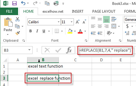
#1 To replace 4 characters in B1 cell with a new text string and starting with 7^th character in old_text text, just using formula:

=REPLACE(B1,7,4," replace")

#2 you can use the Excel’s REPLACE function to replace unwanted text string in a cell with another text string or empty string.

When you copied or imported data from the external application (such as: Microsoft word), it may include unwanted characters or text string along with the good data. At this time, you can use the REPLACE function to remove it.

For example, if you want to replace the first character of the text string “#158” with a dollar sign, you can use the below REPLACE formula:

=REPLACE(B1,1,1,"$")

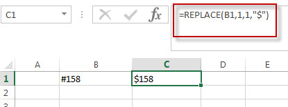
You will get the result as: $158 in the above formula.

More Replace Formula Examples in Excel

Combining the Replace function with Text function in Excel
we can use Replace function in combination with Text function to replace date characters that are part of the text string in excel…
Excel Replace function with numeric values
how to replace a numeric characters within a text string using another numeric characters. This post will guide you how to use REPLACE function to replace numeric characters using another numeric characters in one text string….
Combining the Replace Function with FIND Function to Remove Text
If you want to remove the characters before the hyphen character, then you need use FIND function to get the position of hyphen in the text, then combine with the REPLACE function …
Excel Replace Function Remove Text String
If you want to remove the characters before the hyphen character, then you need use FIND function to get the position of hyphen in the text, then combine with the REPLACE function…
The difference between Replace function and Substitute function
there are two similar functions to replace text string in Excel. They are REPLACE and SUBSTITUTE functions. What’s the difference between REPLACE function and SUBSTITUTE function in excel 2013? This post will introduce the difference between those two function in excel…

Excel Replace function
The Excel DATE function returns the serial number for a date.The syntax of the DATE function is as below:= DATE (year, month, day) …
Excel Substitute function
The Excel SUBSTITUTE function replaces a new text string for an old text string in a text string. ….
Excel FIND function
The Excel FIND function returns the position of the first text string (substring) from the first character of the second text string.The FIND function is a build-in function in Microsoft Excel and it is categorized as a Text Function.The syntax of the FIND function is as below:= FIND (find_text, within_text,[start_num])…

Frequently Asked Questions

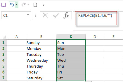
Question 1:

I have a number of cell that contains day name of the week, and I want to change the full day name of the week to the abbreviation of day name. How to achieve this requirement in excel.

Answer: you can use Text function or replace function to achieve it. I will show you how to use REPLACE function to change the full day name of the week, just entering the following formula to the cell B1,

=REPLACE(B1,4,6,"")

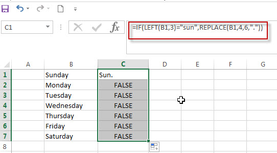
Question2: I have a data in the excel worksheet, and I want to check if the first three characters are “sun” in a cell and then replace others characters with “.”, just keep “sun” characters in this cell. How to achieve this using excel formula.

Answer: To achieve this, you need to use Replace function with IF function and LEFT function, using IF function to check the first characters if it is equal to “sun”, if TRUE, then call REPLACE function to remove the rest characters with “.”. And Using LEFT function to get the first three characters of a cell.

So we can write down the following formula:

=IF(LEFT(B1,3)="sun",REPLACE(B1,4,6,"."))

More reading: Using Find and Replace Tool to replace text in Excel

Источник

Find

Replace

Find

Replace

Need more help?

Recommended articles

How to Replace Text in Excel with the REPLACE function (2023)

Replacing characters in text with the REPLACE function

Step 1: Old text

Step 2: Start num

Step 3: Num chars

Step 4: New text

PRO TIP: Length of num_chars vs new_text

Replacing text strings with the SUBSTITUTE function

Step 1: Text

Step 2: Old text

Step 3: New text

Step 4: Instance num

The difference between REPLACE and SUBSTITUTE

Replace text using Find and Replace

That’s it – Now what?

Other resources

Description

Syntax

Excel REPLACE Function Examples

More Replace Formula Examples in Excel

Frequently Asked Questions