Excel removing duplicates column

Sometimes duplicate data is useful, sometimes it just makes it harder to understand your data. Use conditional formatting to find and highlight duplicate data. That way you can review the duplicates and decide if you want to remove them.

1. Select the cells you want to check for duplicates.

   Note: Excel can’t highlight duplicates in the Values area of a PivotTable report.

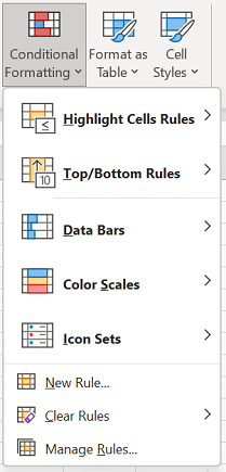
2. Click Home > Conditional Formatting > Highlight Cells Rules > Duplicate Values.

   

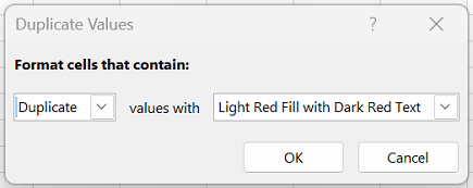
3. In the box next to values with, pick the formatting you want to apply to the duplicate values, and then click OK.

   ​​​​​​​

Remove duplicate values

When you use the Remove Duplicates feature, the duplicate data will be permanently deleted. Before you delete the duplicates, it’s a good idea to copy the original data to another worksheet so you don’t accidentally lose any information.

1. Select the range of cells that has duplicate values you want to remove.

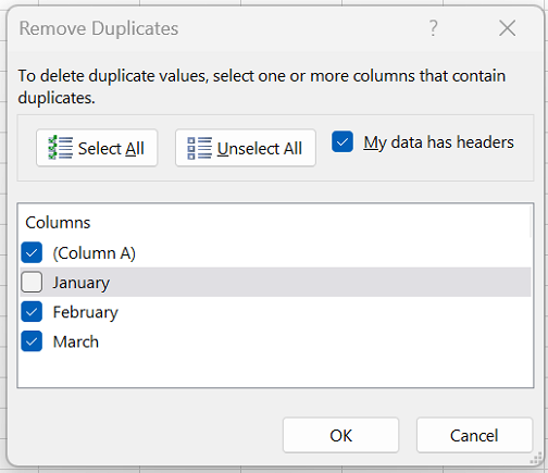
2. Click Data > Remove Duplicates, and then Under Columns, check or uncheck the columns where you want to remove the duplicates.

   

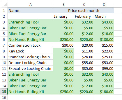
   For example, in this worksheet, the January column has price information I want to keep.

   

   So, I unchecked January in the Remove Duplicates box.

   

3. Click OK.

Note: The counts of duplicate and unique values given after removal may include empty cells, spaces, etc. 

Need more help?

​​​​​​​

Filter for unique values or remove duplicate values

In Excel, there are several ways to filter for unique values—or remove duplicate values:

• To filter for unique values, click Data > Sort & Filter > Advanced.
  

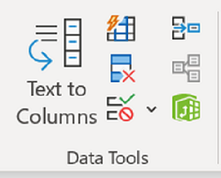
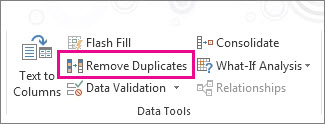
• To remove duplicate values, click Data > Data Tools > Remove Duplicates.
  

• To highlight unique or duplicate values, use the Conditional Formatting command in the Style group on the Home tab.

Filtering for unique values and removing duplicate values are two similar tasks, since the objective is to present a list of unique values. There is a critical difference, however: When you filter for unique values, the duplicate values are only hidden temporarily. However, removing duplicate values means that you are permanently deleting duplicate values.

A duplicate value is one in which all values in at least one row are identical to all of the values in another row. A comparison of duplicate values depends on the what appears in the cell—not the underlying value stored in the cell. For example, if you have the same date value in different cells, one formatted as «3/8/2006» and the other as «Mar 8, 2006», the values are unique.

Check before removing duplicates: Before removing duplicate values, it’s a good idea to first try to filter on—or conditionally format on—unique values to confirm that you achieve the results you expect.

Follow these steps:

1. Select the range of cells, or ensure that the active cell is in a table.

2. Click Data > Advanced (in the Sort & Filter group).

   

3. In the Advanced Filter popup box, do one of the following:

To filter the range of cells or table in place:

• Click Filter the list, in-place.

To copy the results of the filter to another location:

• Click Copy to another location.

• In the Copy to box, enter a cell reference.

• Alternatively, click Collapse Dialog to temporarily hide the popup window, select a cell on the worksheet, and then click Expand .

• Check the Unique records only, then click OK.

The unique values from the range will copy to the new location.

When you remove duplicate values, the only effect is on the values in the range of cells or table. Other values outside the range of cells or table will not change or move.  When duplicates are removed, the first occurrence of the value in the list is kept, but other identical values are deleted. 

Because you are permanently deleting data, it’s a good idea to copy the original range of cells or table to another worksheet or workbook before removing duplicate values.

Follow these steps:

1. Select the range of cells, or ensure that the active cell is in a table.

2. On the Data tab, click Remove Duplicates (in the Data Tools group).

   

3. Do one or more of the following:

   • Under Columns, select one or more columns.

   • To quickly select all columns, click Select All.

   • To quickly clear all columns, click Unselect All.

     If the range of cells or table contains many columns and you want to only select a few columns, you may find it easier to click Unselect All, and then under Columns, select those columns.

     Note: Data will be removed from all columns, even if you don’t select all the columns at this step. For example, if you select Column1 and Column2, but not Column3, then the “key” used to find duplicates is the value of BOTH Column1 & Column2.  If a duplicate is found in those columns, then the entire row will be removed, including other columns in the table or range.

4. Click OK, and a message will appear to indicate how many duplicate values were removed, or how many unique values remain. Click OK to dismiss this message.

5. Undo the change by click Undo (or pressing Ctrl+Z on the keyboard).

Note: You cannot conditionally format fields in the Values area of a PivotTable report by unique or duplicate values.

Quick formatting

Follow these steps:

1. Select one or more cells in a range, table, or PivotTable report.

2. On the Home tab, in the Style group, click the small arrow for Conditional Formatting, and then click Highlight Cells Rules, and select Duplicate Values.
   

3. Enter the values that you want to use, and then choose a format.

Advanced formatting

Follow these steps:

1. Select one or more cells in a range, table, or PivotTable report.

2. On the Home tab, in the Styles group, click the arrow for Conditional Formatting, and then click Manage Rules to display the Conditional Formatting Rules Manager popup window.
   

3. Do one of the following:

   • To add a conditional format, click New Rule to display the New Formatting Rule popup window.

   • To change a conditional format, begin by ensuring that the appropriate worksheet or table has been chosen in the Show formatting rules for list. If necessary, choose another range of cells by clicking Collapse button in the Applies to popup window temporarily hide it. Choose a new range of cells on the worksheet, then expand the popup window again . Select the rule, and then click Edit rule to display the Edit Formatting Rule popup window.

4. Under Select a Rule Type, click Format only unique or duplicate values.

5. In the Format all list of Edit the Rule Description, choose either unique or duplicate.

6. Click Format to display the Format Cells popup window.

7. Select the number, font, border, or fill format that you want to apply when the cell value satisfies the condition, and then click OK. You can choose more than one format. The formats that you select are displayed in the Preview panel.

In Excel for the web, you can remove duplicate values.

Remove duplicate values

When you remove duplicate values, the only effect is on the values in the range of cells or table. Other values outside the range of cells or table will not change or move. When duplicates are removed, the first occurrence of the value in the list is kept, but other identical values are deleted.

Important: You can always click Undo to get back your data after you have removed the duplicates. That being said, it’s a good idea to copy the original range of cells or table to another worksheet or workbook before removing duplicate values.

Follow these steps:

1. Select the range of cells, or ensure that the active cell is in a table.

2. On the Data tab, click Remove Duplicates .

3. In the Remove Duplicates dialog box, unselect any columns where you don’t want to remove duplicate values.

   Note: Data will be removed from all columns, even if you don’t select all the columns at this step. For example, if you select Column1 and Column2, but not Column3, then the “key” used to find duplicates is the value of BOTH Column1 & Column2.  If a duplicate is found in Column1 and Column2, then the entire row will be removed, including data from Column3.

4. Click OK, and a message will appear to indicate how many duplicate values were removed. Click OK to dismiss this message.

Note: If you want to get back your data, simply click Undo (or press Ctrl+Z on the keyboard).

Need more help?

You can always ask an expert in the Excel Tech Community or get support in the Answers community.

See Also

Count unique values among duplicates

Duplicate values in your data can be a big problem! It can lead to substantial errors and over estimate your results.

But finding and removing them from your data is actually quite easy in Excel.

In this tutorial, we are going to look at 7 different methods to locate and remove duplicate values from your data.

Video Tutorial

What Is A Duplicate Value?

Duplicate values happen when the same value or set of values appear in your data.

For a given set of data you can define duplicates in many different ways.

In the above example, there is a simple set of data with 3 columns for the Make, Model and Year for a list of cars.

1. The first image highlights all the duplicates based only on the Make of the car.
2. The second image highlights all the duplicates based on the Make and Model of the car. This results in one less duplicate.
3. The second image highlights all the duplicates based on all columns in the table. This results in even less values being considered duplicates.

The results from duplicates based on a single column vs the entire table can be very different. You should always be aware which version you want and what Excel is doing.

Find And Remove Duplicate Values With The Remove Duplicates Command

Removing duplicate values in data is a very common task. It’s so common, there’s a dedicated command to do it in the ribbon.

Select a cell inside the data which you want to remove duplicates from and go to the Data tab and click on the Remove Duplicates command.

Excel will then select the entire set of data and open up the Remove Duplicates window.

1. You then need to tell Excel if the data contains column headers in the first row. If this is checked, then the first row of data will be excluded when finding and removing duplicate values.
2. You can then select which columns to use to determine duplicates. There are also handy Select All and Unselect All buttons above you can use if you’ve got a long list of columns in your data.

When you press OK, Excel will then remove all the duplicate values it finds and give you a summary count of how many values were removed and how many values remain.

This command will alter your data so it’s best to perform the command on a copy of your data to retain the original data intact.

Find And Remove Duplicate Values With Advanced Filters

There is also another way to get rid of any duplicate values in your data from the ribbon. This is possible from the advanced filters.

Select a cell inside the data and go to the Data tab and click on the Advanced filter command.

This will open up the Advanced Filter window.

1. You can choose to either to Filter the list in place or Copy to another location. Filtering the list in place will hide rows containing any duplicates while copying to another location will create a copy of the data.
2. Excel will guess the range of data, but you can adjust it in the List range. The Criteria range can be left blank and the Copy to field will need to be filled if the Copy to another location option was chosen.
3. Check the box for Unique records only.

Press OK and you will eliminate the duplicate values.

Advanced filters can be a handy option for getting rid of your duplicate values and creating a copy of your data at the same time. But advanced filters will only be able to perform this on the entire table.

Find And Remove Duplicate Values With A Pivot Table

Pivot tables are just for analyzing your data, right?

You can actually use them to remove duplicate data as well!

You won’t actually be removing duplicate values from your data with this method, you will be using a pivot table to display only the unique values from the data set.

First, create a pivot table based on your data. Select a cell inside your data or the entire range of data ➜ go to the Insert tab ➜ select PivotTable ➜ press OK in the Create PivotTable dialog box.

With the new blank pivot table add all fields into the Rows area of the pivot table.

You will then need to change the layout of the resulting pivot table so it’s in a tabular format. With the pivot table selected, go to the Design tab and select Report Layout. There are two options you will need to change here.

1. Select the Show in Tabular Form option.
2. Select the Repeat All Item Labels option.

You will also need to remove any subtotals from the pivot table. Go to the Design tab ➜ select Subtotals ➜ select Do Not Show Subtotals.

You now have a pivot table that mimics a tabular set of data!

Pivot tables only list unique values for items in the Rows area, so this pivot table will automatically remove any duplicates in your data.

Find And Remove Duplicate Values With Power Query

Power Query is all about data transformation, so you can be sure it has the ability to find and remove duplicate values.

Select the table of values which you want to remove duplicates from ➜ go to the Data tab ➜ choose a From Table/Range query.

Remove Duplicates Based On One Or More Columns

With Power Query, you can remove duplicates based on one or more columns in the table.

You need to select which columns to remove duplicates based on. You can hold Ctrl to select multiple columns.

Right click on the selected column heading and choose Remove Duplicates from the menu.

You can also access this command from the Home tab ➜ Remove Rows ➜ Remove Duplicates.

= Table.Distinct(#"Previous Step", {"Make", "Model"})

If you look at the formula that’s created, it is using the Table.Distinct function with the second parameter referencing which columns to use.

Remove Duplicates Based On The Entire Table

To remove duplicates based on the entire table, you could select all the columns in the table then remove duplicates. But there is a faster method that doesn’t require selecting all the columns.

There is a button in the top left corner of the data preview with a selection of commands that can be applied to the entire table.

Click on the table button in the top left corner ➜ then choose Remove Duplicates.

= Table.Distinct(#"Previous Step")

If you look at the formula that’s created, it uses the same Table.Distinct function with no second parameter. Without the second parameter, the function will act on the whole table.

Keep Duplicates Based On A Single Column Or On The Entire Table

In Power Query, there are also commands for keeping duplicates for selected columns or for the entire table.

Follow the same steps as removing duplicates, but use the Keep Rows ➜ Keep Duplicates command instead. This will show you all the data that has a duplicate value.

Find And Remove Duplicate Values Using A Formula

You can use a formula to help you find duplicate values in your data.

First you will need to add a helper column that combines the data from any columns which you want to base your duplicate definition on.

= [@Make] & [@Model] & [@Year]

The above formula will concatenate all three columns into a single column. It uses the ampersand operator to join each column.

= TEXTJOIN("", FALSE , CarList[@[Make]:[Year]])

If you have a long list of columns to combine, you can use the above formula instead. This way you can simply reference all the columns as a single range.

You will then need to add another column to count the duplicate values. This will be used later to filter out rows of data that appear more than once.

= COUNTIFS($E$3:E3, E3)

Copy the above formula down the column and it will count the number of times the current value appears in the list of values above.

If the count is 1 then it’s the first time the value is appearing in the data and you will keep this in your set of unique values. If the count is 2 or more then the value has already appeared in the data and it is a duplicate value which can be removed.

Add filters to your data list.

• Go to the Data tab and select the Filter command.
• Use the keyboard shortcut Ctrl + Shift + L.

Now you can filter on the Count column. Filtering on 1 will produce all the unique values and remove any duplicates.

You can then select the visible cells from the resulting filter to copy and paste elsewhere. Use the keyboard shortcut Alt + ; to select only the visible cells.

Find And Remove Duplicate Values With Conditional Formatting

With conditional formatting, there’s a way to highlight duplicate values in your data.

Just like the formula method, you need to add a helper column that combines the data from columns. The conditional formatting doesn’t work with data across rows, so you’ll need this combined column if you want to detect duplicates based on more than one column.

Then you need to select the column of combined data.

To create the conditional formatting, go to the Home tab ➜ select Conditional Formatting ➜ Highlight Cells Rules ➜ Duplicate Values.

This will open up the conditional formatting Duplicate Values window.

1. You can select to either highlight Duplicate or Unique values.
2. You can also choose from a selection of predefined cell formats to highlight the values or create your own custom format.

Warning: The previous methods to find and remove duplicates considers the first occurrence of a value as a duplicate and will leave it intact. However, this method will highlight the first occurrence and will not make any distinction.

With the values highlighted, you can now filter on either the duplicate or unique values with the filter by color option. Make sure to add filters to your data. Go to the Data tab and select the Filter command or use the keyboard shortcut Ctrl + Shift + L.

1. Click on the filter toggle.
2. Select Filter by Color in the menu.
3. Filter on the color used in the conditional formatting to select duplicate values or filter on No Fill to select unique values.

You can then select just the visible cells with the keyboard shortcut Alt + ;.

Find And Remove Duplicate Values Using VBA

There is a built in command in VBA for removing duplicates within list objects.

Sub RemoveDuplicates() Dim DuplicateValues As Range Set DuplicateValues = ActiveSheet.ListObjects("CarList").Range DuplicateValues.RemoveDuplicates Columns:=Array(1, 2, 3), Header:=xlYes End Sub

The above procedure will remove duplicates from an Excel table named CarList.

Columns:=Array(1, 2, 3)

The above part of the procedure will set which columns to base duplicate detection on. In this case it will be on the entire table since all three columns are listed.

Header:=xlYes

The above part of the procedure tells Excel the first row in our list contains column headings.

You will want to create a copy of your data before running this VBA code, as it can’t be undone after the code runs.

Conclusions

Duplicate values in your data can be a big obstacle to a clean data set.

Thankfully, there are many options in Excel to easily remove those pesky duplicate values.

So, what’s your go to method to remove duplicates?

Watch Video – How to Find and Remove Duplicates in Excel

With a lot of data…comes a lot of duplicate data. 

Duplicates in Excel can cause a lot of troubles. Whether you import data from a database, get it from a colleague, or collate it yourself, duplicates data can always creep in. And if the data you are working with is huge, then it becomes really difficult to find and remove these duplicates in Excel.

In this tutorial, I’ll show you how to find and remove duplicates in Excel.

Find and Highlight Duplicates in Excel

Duplicates in Excel can come in many forms. You can have it in a single column or multiple columns. There may also be a duplication of an entire row.

Finding and Highlight Duplicates in a Single Column in Excel

Conditional Formatting makes it simple to highlight duplicates in Excel.

Here is how to do it:

• Select the data in which you want to highlight the duplicates.

• Go to Home –> Conditional Formatting –> Highlight Cell Rules –> Duplicate Values.

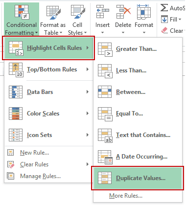
• In the Duplicate Values dialog box, select Duplicate in the drop down on the left, and specify the format in which you want to highlight the duplicate values. You can choose from the ready-made format options (in the drop down on the right), or specify your own format.

• This will highlight all the values that have duplicates.

Quick Tip: Remember to check for leading or trailing spaces. For example, “John” and “John ” are considered different as the latter has an extra space character in it. A good idea would be to use the TRIM function to clean your data.

Finding and Highlight Duplicates in Multiple Columns in Excel

If you have data that spans multiple columns and you need to look for duplicates in it, the process is exactly the same as above.

Here is how to do it:

• Select the data.
• Go to Home –> Conditional Formatting –> Highlight Cell Rules –> Duplicate Values.
• In the Duplicate Values dialog box, select Duplicate in the drop down on the left, and specify the format in which you want to highlight the duplicate values.
• This will highlight all the cells that have duplicates value in the selected data set.

Finding and Highlighting Duplicate Rows in Excel

Finding duplicate data and finding duplicate rows of data are 2 different things. Have a look:

Finding duplicate rows is a bit more complex than finding duplicate cells.

Here are the steps:

• In an adjacent column, use the following formula:
  =A2&B2&C2&D2
  Drag this down for all the rows. This formula combines all the cell values as a single string. (You can also use the CONCATENATE function to combine text strings)

By doing this, we have created a single string for each row. If there are duplicate rows in this dataset, then these strings would be exactly the same for it.

Now that we have the combined strings for each row, we can use conditional formatting to highlight duplicate strings. A highlighted string implies that the row has a duplicate.

Here are the steps to highlight duplicate strings:

• Select the range that has the combined strings (E2:E16 in this example).
• Go to Home –> Conditional Formatting –> Highlight Cell Rules –> Duplicate Values.
• In the Duplicate Values dialog box, make sure Duplicate is selected and then specify the color in which you want to highlight the duplicate values.

This would highlight the duplicate values in column E.

In the above approach, we have highlighted only the strings that we created.

But what if you want to highlight all the duplicate rows (instead of highlighting cells in one single column)?

Here are the steps to highlight duplicate rows:

• In an adjacent column, use the following formula:
  =A2&B2&C2&D2
  Drag this down for all the rows. This formula combines all the cell values as a single string.

• Select the data A2:D16.
• With the data selected, go to Home –> Conditional Formatting –> New Rule.

• In the ‘New Formatting Rule’ dialog box, click on ‘Use a formula to determine which cells to format’.
• In the field below, use the following COUNTIF function:
  =COUNTIF($E$2:$E$16,$E2)>1

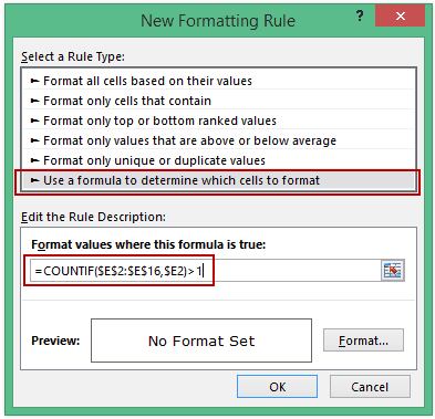
• Select the format and click OK.

This formula would highlight all the rows that have a duplicate.

Remove Duplicates in Excel

In the above section, we learned how to find and highlight duplicates in excel. In this section, I will show you how to get rid of these duplicates.

Remove Duplicates from a Single Column in Excel

If you have the data in a single column and you want to remove all the duplicates, here are the steps:

• Select the data.
• Go to Data –> Data Tools –> Remove Duplicates.
• In the Remove Duplicates dialog box:
  • If your data has headers, make sure the ‘My data has headers’ option is checked.
  • Make sure the column is selected (in this case there is only one column).

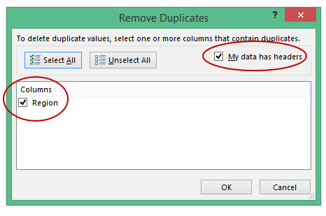
• Click OK.

This would remove all the duplicate values from the column, and you would have only the unique values.

CAUTION: This alters your data set by removing duplicates. Make sure you have a back-up of the original data set. If you want to extract the unique values at some other location, copy this dataset to that location and then use the above-mentioned steps. Alternatively, you can also use Advanced Filter to extract unique values to some other location.

Remove Duplicates from Multiple Columns in Excel

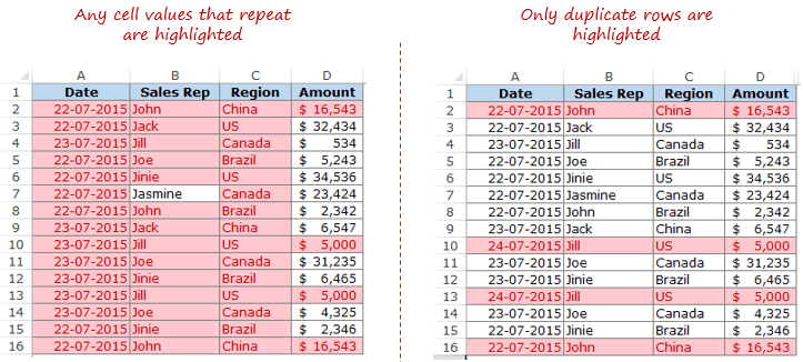
Suppose you have the data as shown below:

In the above data, row #2 and #16 have the exact same data for Sales Rep, Region, and Amount, but different dates (same is the case with row #10 and #13). This could be an entry error where the same entry has been recorded twice with different dates.

To delete the duplicate row in this case:

• Select the data.
• Go to Data –> Data Tools –> Remove Duplicates.
• In the Remove Duplicates dialog box:
  • If your data has headers, make sure the ‘My data has headers’ option is checked.
  • Select all the columns except the Date column.

• Click OK.

This would remove the 2 duplicate entries.

NOTE: This keeps the first occurrence and removes all the remaining duplicate occurrences.

Remove Duplicate Rows in Excel

To delete duplicate rows, here are the steps:

• Select the entire data.
• Go to Data –> Data Tools –> Remove Duplicates.
• In the Remove Duplicates dialog box:
  • If your data has headers, make sure the ‘My data has headers’ option is checked.
  • Select all the columns.

• Click OK.

Use the above-mentioned techniques to clean your data and get rid of duplicates.

You May Also Like the Following Excel Tutorials:

• 10 Ways to Clean Data in Excel Spreadsheets.
• Remove Leading and Trailing Spaces in Excel.
• 24 Daily Excel Issues and their Quick Fixes.
• How to Find Merged Cells in Excel.

Explanation

Remove Duplicates is a popular Excel tool that lets the user remove duplicates from a column or a set of columns. Learn with this tutorial how to remove duplicates in Excel Online and Excel Desktop.

When applied to a range with more than one column, the Remove Duplicates tool will remove the entire row of the duplicate value. 

We can access the Remove Duplicates tool by first selecting the desired range for duplicates removal, then navigating to the Data ribbon in Excel, and then clicking Remove Duplicates. See more on how to identify and remove duplicates here.

Please note that for each set of duplicate values, Remove Duplicates will keep the first duplicate value, and remove the rest.

Example

Let’s see an example of removing duplicates in a single column of names:

Note that Excel identified that the first cell is the header of your column, therefore excluded it from the range for duplicate removal. You can untick the “My data has headers” if you wish to include the first cell as well. 

Removing Duplicates in a range of more than one column

When removing duplicates in a range with multiple columns, we have two options:

First option – Remove duplicates based on one column. This will look for duplicates in the selected column, but remember that it removes the entire row!

Let’s see an example of this;

As you can see, we had duplicates in number 6,7,8 – And they were removed, while the first rows were kept intact.

Second option – Remove duplicates based on a number of columns. This option will look for duplicates in each of the selected columns, and remove any row in which ALL Columns contain a duplicate value!

For example:

Easy, right?

Now, let’s practice a little bit. 

Click here to download a practice spreadsheet for the Remove Duplicates tool in Excel!