Presentation on theme: «Microsoft Excel.»— Presentation transcript:
1
Microsoft Excel
2
How to Use Tutorial Step 1> The next page will show you the table of contents Step 2> Use the mouse and click on the topic links to begin learning Step 3> You can learn at your own pace, click on the Action buttons to review the material as much as you need to. Step 4> Once you become familiar with this application you can use this tutorial as a reference tool. To begin learning click on this button>>
3
Table of Contents 1_ Introduction to Excel
2_ Overview of the Excel Screen 3_ The Excel Menus: File Menu Edit Menu Insert Menu Format Menu View Menu Help Menu and Office Assistant 4_ Excel Worksheets 5_ Entering Formulas and Data 6_ Formatting Workbooks 7_ Charts 8_ Freezing Panes 9_ Printing 10_ Keyboard Shortcuts
4
Introduction to Excel Excel is a computer program used to create electronic spreadsheets. Within Excel, users can organize data, create charts, and perform calculations. Excel is a convenient program because it allows the user to create large spreadsheets, reference information from other spreadsheets, and it allows for better storage and modification of information. Excel operates like other Microsoft (MS) Office programs and has many of the same functions and shortcuts of other MS programs.
5
Overview of the Excel Screen
Before working with Excel, it is essential to first become familiar with the Excel screen. The following will help you to recognize the various parts of an Excel screen and their functions. The Title bar is located at the very top of the screen. The Title bar displays the name of the workbook you are currently using. The Menu bar is located just below the Title bar. The Menu bar is used to give instructions to the program.
6
Overview of the Excel Screen
Toolbars provide shortcuts to menu commands. There are many different toolbars and the user can choose which toolbars are shown on the screen. To enable more toolbars go to “View” on the Menu bar, select Toolbars, then select which toolbar you wish to add to the screen. The Standard Toolbar provides shortcuts to the File Menu, as well as mathematical functions, chart creation, and sorting. The Formatting Toolbar provides shortcuts to font formatting as well as mathematical functions. The Status Toolbar allows the user to view if the current worksheet is ready to enter data.
7
Overview of the Excel Screen
Microsoft Excel consists of workbooks. Within each workbook, there is an infinite number of worksheets. Each worksheet contains columns and rows. Where a column and a row intersect is called the cell. For example, cell B6 is located where column B and row 6 meet. You enter your data into the cells on the worksheet. The tabs at the bottom of the screen represent different worksheets within a workbook. You can use the scrolling buttons on the left to bring other worksheets into view.
8
Overview of the Excel Screen
The Name Box indicates what cell you are in. This cell is called the “active cell.” This cell is highlighted by a black box. The “=” is used to edit your formula on your selected cell. The Formula Bar indicates the contents of the cell selected. If you have created a formula, then the formula will appear in this space.
9
File Menu When first opening Excel a worksheet will automatically appear. However, if you desire to open a file that you previously worked on go to the “File” option located in the top left corner. Select “Open.” To create a new worksheet go to the “File” option and select “New.” To save the work created go to the “File” option and select “Save.” To close an existing worksheet go to the “File” option and select “Close.” To exit the program entirely go to the “File” option and select “Exit.”
10
Edit Menu Among the many functions, the Edit Menu allows you to make changes to any data that was entered. You can: Undo mistakes made. Excel allows you to undo up to the last 16 moves you made. Cut, copy, or paste information. Find information in an existing workbook Replace existing information.
11
Insert Menu The Insert Menu allows you to:
Add new worksheets, rows, and columns to an existing. You can also insert charts, pictures, and objects onto your worksheet.
12
Format Menu You can change the colors, borders, sizes, alignment, and font of a certain cell by going to the “Cell” option in the Format Menu.
13
Format Menu You can change row and column width and height in the “Row” and “Column” options. You can rename worksheets and change their order in the “Sheet” option. The “AutoFormat” option allows you to apply pre-selected colors, fonts, and sizes to entire worksheets.
14
View Menu The View menu allows you different options of viewing your work. You can enable a Full Screen view that changes the view to include just the worksheet and Menu bar. You can zoom in on your worksheet to focus on a smaller portion.
15
View Menu You can change the view of your work so that it is page by page. You can insert Headers and Footers to your work. You can add comments about a specific cell for future reference.
16
Help Menu and Office Assistant
The Help Menu is used to answer any questions you many have with the program. You can also get online assistance if it is needed. The Office Assistant is a shortcut to the Help Menu. You can ask the assistant a question and it will take you directly to an index of topics that will help you solve your problem.
17
Excel Worksheets With Excel, you will be working with different worksheets within a workbook. Often times it is necessary to name the different worksheets so that it is easier to find them. To do so you must: 1_Double click to highlight an existing worksheet 2_Type in what you would like to rename the worksheet
18
Entering Formulas ADDITION FORMULAS
When entering numerical data, you can command Excel to do any mathematical function. Start each formula with an equal sign (=). To enter the same formulas for a range of cells, use the colon sign “:” ADDITION FORMULAS To add cells together use the “+” sign. To sum up a series of cells, highlight the cells, then click the auto sum button. The answer will appear at the bottom of the highlighted box.
19
Entering Formulas SUBTRACTION FORMULAS
To subtract cells, use the “-” sign. DIVISION FORMULAS To divide cells, use the “/” sign. MULTIPLICATION FORMULAS To multiply cells, use the “*” sign.
20
Tips for Entering Data To highlight a series of cells click and drag the mouse over the desired area. To move a highlighted area, click on the border of the box and drag the box to the desired location. You can sort data (alphabetically, numerically, etc). By highlighting cells then pressing the sort shortcut key.
21
Tips for Entering Data You can cut and paste to move data around.
To update your worksheets, you can use the find and replace action (under the Edit Menu). To change the order of worksheets, click and drag the worksheet tab to the desired order.
22
Formatting Workbooks To add borders to cells, you can select from various border options. To add colors to text or cells, you can select the text color option or the cell fill option, then select the desired color. To change the alignment of the cells, highlight the desired cells and select any of the three alignment options.
23
Formatting Workbooks To check the spelling of your data, highlight the desired cells and click on the spell check button. When entering dollar amounts, you can select the cells you desire to be currency formatted, then click on the “$” button to change the cells. You can bold, italicize, or underline any information in the cells, as well as change the styles and fonts of those cells.
24
Creating Charts With the Excel program you can create charts with the “Chart Wizard.” Step 1: Choose a chart type. Step 2: Highlight the data that you wish to be included in the chart.
25
Creating Charts Step 3: Change chart options. Here you can name the chart and the axes, change the legend, label the data points, and many other options. Step 4: Choose a location for the chart.
26
Freezing Panes If you need the information in one column to freeze, while still being able to scroll through the rest of the data follow these instructions: Step 1: Highlight a specific column. Step 2: Go to the Window Menu and click “Freeze Panes.” Step 3: The cells to the left of the highlighted column should be frozen while you are still able to scroll about the rest of the worksheet (Notice that column A remains while column H is next to it).
27
Printing When printing a worksheet you have a few options.
You can go to “Page Setup” to change the features of your work (the margins, the paper size, the tabs, etc.) This will affect how your project will be printed.
28
Printing You can select “Print Area,” which allows you to only print a highlighted area. You can preview your printing job by selecting “Print Preview.” Finally, you can print your job by going to the File Menu and selecting “Print,” or you can use the shortcut button.
29
Keyboard Shortcuts Here are some basic keyboard shortcuts:
Shift + arrow key = highlight information CTLR + A = Select All CTRL + C = Copy Information CTRL + X = Cut Information CTRL + V = Paste Information CTRL + Z = Undo Information HOME = Move to the beginning of the worksheet
30
Notes to the teacher: This curriculum was designed so that it could be easily modified by the teacher. The teacher can add slides at any point in the curriculum depending on the level of computer literacy of the students. The Basic Outline of the curriculum is to be used as a guidance tool and will help the teacher create a syllabus for the class being taught. Slides that are blank are topics we deemed important but not necessary to have included in the curriculum. These slides were considered advanced topics. (please ignore if there are no blank slides) You can choose to add content to these slides or to delete them.
Слайд 1
Описание слайда:
Презентацию подготовила:
Презентацию подготовила:
Студентка 103 группы лечебного факультета
Марочкина А.Н.
Преподаватель:
Колпакова М.А.
Слайд 2
Описание слайда:
Содержание
Что такое Microsoft Excel
История создания
Создание, загрузка и сохранение фалов — документов.
Окно программы MS Excel
Функции MS Excel
Стандартные функции MS Excel
Заключение
Слайд 3
Описание слайда:
Что такое Microsoft Excel
Microsoft Excel-программа для работы с электронными таблицами, созданная корпорацией Microsoft.
Она предоставляет возможности экономико-статистических расчетов, графические инструменты и, язык макропрограммирования VBA (Visual Basic for Application).
Microsoft Excel входит в состав Microsoft Office и на сегодняшний день Excel является одним из наиболее популярных приложений в мире.
Слайд 4
Описание слайда:
История создания
Какова же история создания столь мощного инструмента для вычислений? Всё началось с того, что в 1982 году компания Microsoft выпустила 1-ый табличный процессор под названием Multiplan, который завоевал огромную популярность среди CP/M систем. Самая 1-ая версия Excel появилась на компьютерах Mac в 1985 году.
А 1-ая версия для Windows стала доступна лишь в ноябре 1987 года. Компания Microsoft решила не останавливаться на достигнутом и год за годом укрепляла свои позиции на рынке и выпускала новые, всё более совершенные версии электронных таблиц Excel.
Слайд 5
Описание слайда:
Создание, загрузка и сохранение фалов — документов.
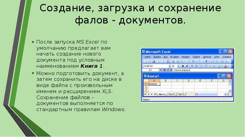
После запуска MS Excel по умолчанию предлагает вам начать создание нового документа под условным наименованием Книга 1.
Можно подготовить документ, а затем сохранить его на диске в виде файла с произвольным именем и расширением.XLS. Сохранение файлов – документов выполняется по стандартным правилам Windows.
Слайд 6
Описание слайда:
Окно программы MS Excel
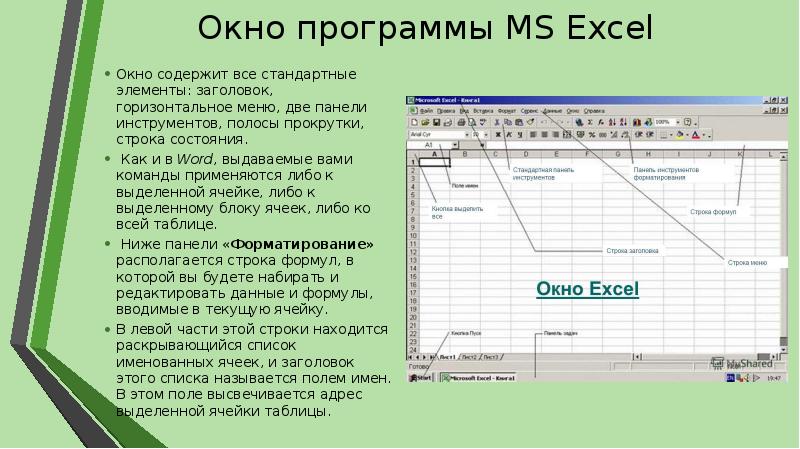
Окно содержит все стандартные элементы: заголовок, горизонтальное меню, две панели инструментов, полосы прокрутки, строка состояния.
Как и в Word, выдаваемые вами команды применяются либо к выделенной ячейке, либо к выделенному блоку ячеек, либо ко всей таблице.
Ниже панели «Форматирование» располагается строка формул, в которой вы будете набирать и редактировать данные и формулы, вводимые в текущую ячейку.
В левой части этой строки находится раскрывающийся список именованных ячеек, и заголовок этого списка называется полем имен. В этом поле высвечивается адрес выделенной ячейки таблицы.
Слайд 7
Описание слайда:
Функции MS Excel
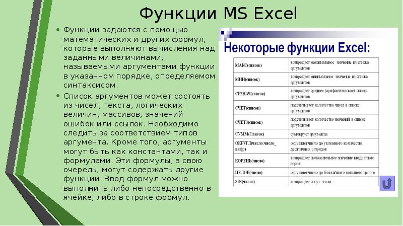
Функции задаются с помощью математических и других формул, которые выполняют вычисления над заданными величинами, называемыми аргументами функции в указанном порядке, определяемом синтаксисом.
Список аргументов может состоять из чисел, текста, логических величин, массивов, значений ошибок или ссылок. Необходимо следить за соответствием типов аргумента. Кроме того, аргументы могут быть как константами, так и формулами. Эти формулы, в свою очередь, могут содержать другие функции. Ввод формул можно выполнить либо непосредственно в ячейке, либо в строке формул.
Слайд 8
Описание слайда:
Стандартные функции MS Excel
Стандартные функции в MS Excel подразделяются на следующие основные группы:
Финансовые;
Функции для работы с датами и временем;
Математические;
Статистические;
Функции для работы со ссылками и массивами;
Функции для работы с базами данных;
Текстовые;
Логические;
Функции для проверки свойств и значений.
Слайд 9
Описание слайда:
Заключение
Программа Microsoft Excel представляет собой электронную таблицу, которая состоит из строк и столбцов.
Запускается эта программа, любым из стандартных способов. В Microsoft Excel файлы можно создавать, загружать и сохранять.
Excel позволяет разделить окно таблицы на два или четыре подокна и одновременно работать с разными частями одной и той же таблицы.
Окно программы по структуре похоже на окно программы MS Word. Оно содержит все стандартные элементы: заголовок, горизонтальное меню, две панели инструментов, полосы прокрутки, строка состояния.
Также в этой программе можно произвести настройку экрана.
Слайд 10
Описание слайда:
СПАСИБО ЗА ВНИМАНИЕ!
1. Excel
EXCEL
FORMULAS, FUNCTIONS, AND OTHER USEFUL
FEATURES
2. Overview
OVERVIEW
• Excel is a spreadsheet, a grid made from columns
and rows. It is a software program that can make
number manipulation easy and somewhat painless.
• The nice thing about using a computer and
spreadsheet is that you can experiment with
numbers without having to RE-DO all the
calculations.
3. Basics of a Spreadsheet
BASICS OF A SPREADSHEET
• Spreadsheets are made up of
• Columns
• Rows
• and their intersections are called cells
4. What is a COLUMN ?
WHAT IS A COLUMN ?
• In a spreadsheet
the COLUMN is
defined as the
vertical space that
is going up and
down the window.
Letters are used to
designate each
COLUMN’S location.
• COLUMN labeled D
is highlighted.
5. What is a row?
WHAT IS A ROW?
• In a spreadsheet
the ROW is defined
as the horizontal
space that is going
across the window.
Numbers are used
to designate each
ROW’S location.
• ROW labeled 4 is
highlighted.
6. What is a CELL ?
WHAT IS A CELL ?
• A CELL is the space
where a row and
column intersect.
Each CELL is
assigned a name
according to its
COLUMN letter and
ROW number.
• In the above
diagram the CELL
labeled C2 is
highlighted.
7. Types of data
TYPES OF DATA
• In each cell there may be the following data
types:
• Labels — (text with no numerical value)
• Number data (constant values)
• Formulas (mathematical equation used to calculate)
Data Types
Examples
Descriptions
LABEL
Name or Wage
or Days
anything that is
just text
CONSTANT
5 or 3.75 or -7.4
any number
FORMULA
=5+3 or = 8*5+3
math equation
8. Labels
LABELS
• Labels are text entries
• Labels help identify what we are talking
about
• Labels do not have a value associated with
them
• Sometimes called ‘headers’
9. Constants
CONSTANTS
• Constants are FIXED
number data
• Constants may refer
to dollars,
percentages, or
number of items (in
this case number of
hours worked within
a certain pay
period).
10. Formulas
FORMULAS
• Formulas are math
equations that CALCULATE
a value to be displayed.
• DO NOT type in the
numbers; type in the
equation.
• It is BEST to Reference as
much data as possible as
opposed to typing data into
equations. That way when
OTHER information changes,
we DO-NOT have to change
the equations or type in
information again.
11. Basic Formulas & Functions
BASIC FORMULAS &
FUNCTIONS
EXCEL 2010
12. Basic Math Functions
BASIC MATH FUNCTIONS
• Math functions built into them. Of the most basic
operations are the standard multiply, divide, add
and subtract.
13. SUM Function
SUM FUNCTION
Definition:
Tips:
• Probably the most
popular function in any
spreadsheet is the SUM
function. The Sum
function takes all of the
values in each of the
specified cells and totals
their values.
• The syntax is: =SUM(first
value, second value, etc)
• Blank cells will return a
value of zero to be
added to the total.
• Text cells can not be
added to a number
and will produce an
error.
14. Sum function
SUM FUNCTION
15. Average Function
AVERAGE FUNCTION
• The average
function finds the
average of the
specified data.
(Simplifies adding all
of the indicated
cells together and
dividing by the total
number of cells.)
16. Max & Min Functions
MAX & MIN FUNCTIONS
• The Max function will return the
largest (max) value in the selected
range of cells. The Min function will
display the smallest value in a
selected set of cells.
17. Count Function
COUNT FUNCTION
• The Count function will return the number of
entries (actually counts each cell that contains
NUMBER DATA) in the selected range of cells.
• Remember: cell that are blank or contain text will
not be counted.
18. IF Function
IF FUNCTION
Definition:
Tips:
• The IF function will
check the logical
condition of a
statement and return
one value if true and a
different value if false.
• The syntax is:
=IF (condition, value-iftrue, value-if-false)
• Until you are used to
writing them, test them
out on multiple cells.
• There are multiple ways
to write an IF statement
to get the same result
19. IF Function
IF FUNCTION
• IF Functions are like
programing — they
provide multiple
answers based on
certain conditions.
20. Data Tools
DATA TOOLS
EXCEL 2010
21. Concatenate function
CONCATENATE FUNCTION
• Concatenate
function — join
several strings into
one text string
Syntax:
• Note: The
concatenate =A1&A2
function does not
automatically leave
a blank space
between words or
other data.
22. Text to Columns
TEXT TO COLUMNS
• Text to Columns – delineate via special characters
or fixed width
23. Removing duplicate values
REMOVING DUPLICATE VALUES
• Removing duplicate values – check for and delete
specific cells with duplicate values
24. Useful Features
USEFUL FEATURES
EXCEL 2010
25. Instantly reveal formulas and general number format of all cells
INSTANTLY REVEAL FORMULAS AND GENERAL
NUMBER FORMAT OF ALL CELLS
• Show all formulas and the general number
format of cells
• Saves you time because you don’t have to
move the cell pointer to check each
formula one-by-one.
26. Keyboard short cut to Instantly reveal formulas
KEYBOARD SHORT CUT TO
INSTANTLY REVEAL FORMULAS
• To do this, just press
the Ctrl key and the
tilde key at the same
time. The tilde is the
squiggly line that is
directly above the
tab key in the upper
left corner of your
keyboard. To change
your worksheet back
to the normal view,
just press the Ctrl and
tilde keys again.
27. Comparing 2 or more Excel spreadsheets simultaneously
COMPARING 2 OR MORE EXCEL SPREADSHEETS
SIMULTANEOUSLY
• You can open two
instances of Excel INSTEAD
of multiple files on top of
each other in the same
Excel application.
• To do this, simply open Excel
by double clicking the icon
on your desktop and open
the first Excel file you want
to use. Minimize this
window and move it to the
right screen. Then go back
to the desktop, double click
the Excel icon once
more, another separate
Excel window will open.
28. Sorting
SORTING
• Arranging data so it’s easy to analyze
• You can sort the data alphabetically, from highest
to lowest, or by a number of additional criteria
(such as cell color)
29. filters
FILTERS
• The Filter is a quick and easy way to find and work
with a subset of data in a range of cells.
30. Tables
TABLES
• To make managing and analyzing a group of
related data easier, you can turn a range of cells
into a Microsoft Office Excel table (previously known
as an Excel list). A table typically contains related
data in a series of worksheet rows and columns that
have been formatted as a table. By using the table
features, you can then manage the data in the
table rows and columns independently from the
data in other rows and columns on the worksheet.
31. Elements of an excel table
ELEMENTS OF AN EXCEL TABLE
• Header row By default, a table has a header row.
Every table column has filtering enabled in the
header row so that you can filter or sort your table
data quickly.
32. Elements of an excel table
ELEMENTS OF AN EXCEL TABLE
• Banded rows By default, alternate shading or
banding has been applied to the rows in a table to
better distinguish the data.
33. Elements of an excel table
ELEMENTS OF AN EXCEL TABLE
• Total row You can
add a total row to your
table that provides
access to summary
functions (such as the
AVERAGE, COUNT, or
SUM function). A dropdown list appears in
each total row cell so
that you can quickly
calculate the totals that
you want.
34. Creating a table
CREATING A TABLE
35. Freeze Headers
FREEZE HEADERS
• To freeze a row in your worksheet, highlight the row
where you wish all rows before the highlighted row
to be frozen or locked, go to Window>Freeze Panes
and you will see a line appear across your
worksheet. Everything above the line is frozen and
will remain in view when you scroll down your
worksheet.
36. Set print area
SET PRINT AREA
37. Narrow margins
NARROW MARGINS
38. Shrink to fit
SHRINK TO FIT
39. Pivot Table
PIVOT TABLE
• A Pivot table lets your arrange, sort, and filter a set
of data on the fly so you can analyze it from
different perspectives with minimum effort.
• Start with a data list with a few columns
• Make sure each of the rows have a value of each one of
the columns
40. Excel Cell References Worth Remembering
EXCEL CELL REFERENCES WORTH
REMEMBERING
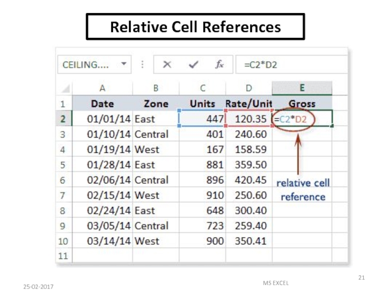
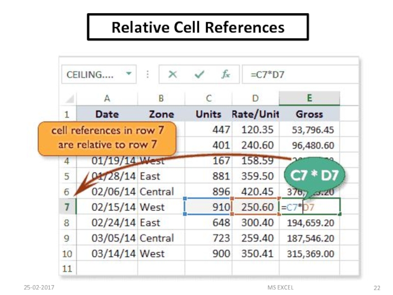
• In Excel formulas, you can refer to
other cells either relatively or
absolutely. When you copy and
paste a formula in Excel, how you
create the references within the
formula tells Excel what to change
in the formula it pastes. The formula
can either change the references
relative to the cell where you’re
pasting it (relative reference), or it
can always refer to a specific cell.
You can also mix relative and
absolute references so that, when
you move or copy a formula, the
row changes but the column does
not, or vice versa.
• Preceding the row and/or column
designators with a dollar sign ($)
specifies an absolute reference in
Excel.
Example
Comment
=A1
Complete relative reference
=$A1
The column is absolute; the row is relative
=A$1
The column is relative; the row is absolute
=$A$1
Complete absolute reference
© 2023 Prezi Inc.
Terms & Privacy Policy
Слайд 2 INTRODUCTION TO
MS EXCEL
Excel is a computer program used to
create electronic spreadsheets.
Within excel user can organize data, create chart and perform calculations.
Excel is a convenient program because it allow user to create large spreadsheets, reference information, and it allows for better storage of information.
Excel operates like other Microsoft(MS) office programs and has many of the same functions and shortcuts of other MS programs.
25-02-2017
MS EXCEL
Слайд 3OVERVIEW OF EXCEL
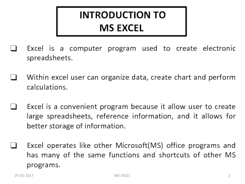
Excel consists of sheets with columns and rows.
Columns
are lettered alphabetically from A to Z and then continuing with AA, AB, AC and so on; rows are numbered 1 to 1,048,576.
Combination of a row and a column makes up a cell address. For example cell D5 is located under column D on row 5.
25-02-2017
MS EXCEL
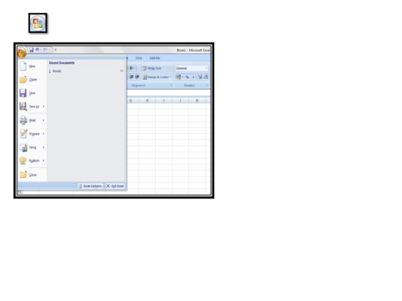
Слайд 5 OFFICE BUTTON
OFFICE BUTTON CONTAINS
NEW-TO OPEN NEW WORKBOOK (CTRL+N)
OPEN-TO OPEN EXISTING
DOCUMENT (CTRL+O)
SAVE-TO SAVE A DOCUMENT (CTRL+S)
SAVE AS-TO SAVE COPY DOCUMENT (F12)
PRINT-TO PRINT A DOCUMENT (CTRL+P)
PREPARE-TO PREPARE DOCUMENT FOR DISTRIBUTION
SEND-TO SEND A COPY OF DOCUMENT TO OTHER PEOPLE
PUBLISH-TO DISTRIBUTE DOCUMENT TO OTHER PEOPLE
CLOSE-TO CLOSE A DOCUMENT (CTRL+W)
25-02-2017
MS EXCEL
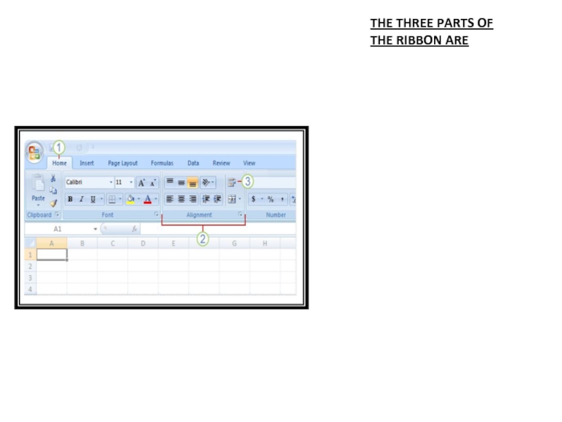
Слайд 6THE THREE PARTS OF THE RIBBON ARE
R I
B B O N
TABS
GROUPS
COMMANDS
25-02-2017
MS EXCEL
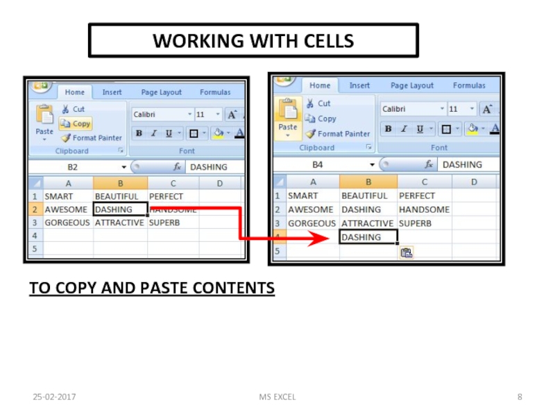
Слайд 8WORKING WITH CELLS
TO COPY AND PASTE CONTENTS
25-02-2017
MS EXCEL
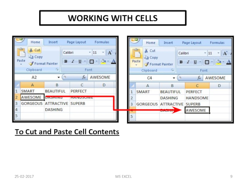
Слайд 9WORKING WITH CELLS
To Cut and Paste Cell Contents
25-02-2017
MS EXCEL
Слайд 10FORMATTING TEXT
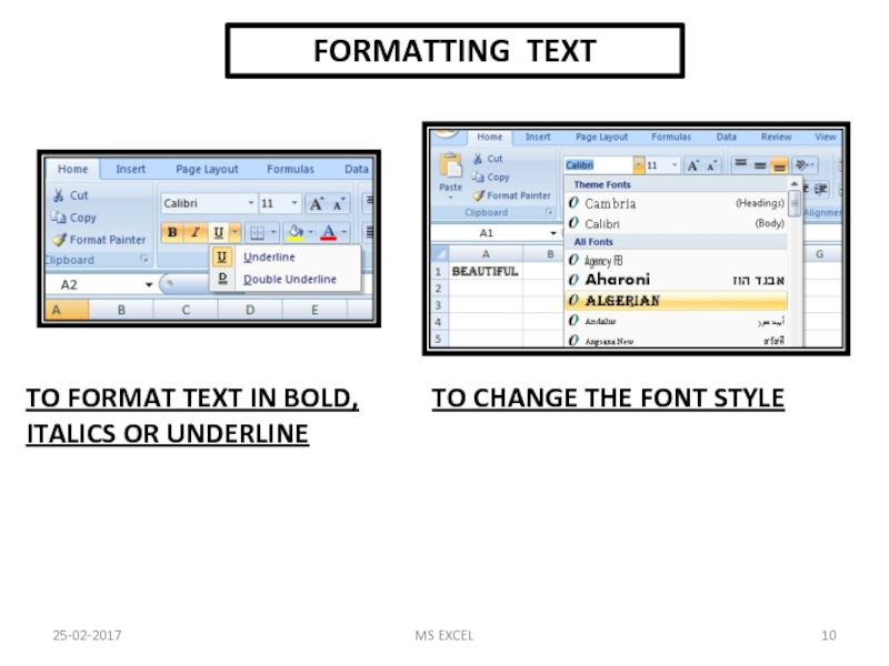
TO FORMAT TEXT IN BOLD, ITALICS OR UNDERLINE
TO CHANGE THE
FONT STYLE
25-02-2017
MS EXCEL
Слайд 11FORMATTING TEXT
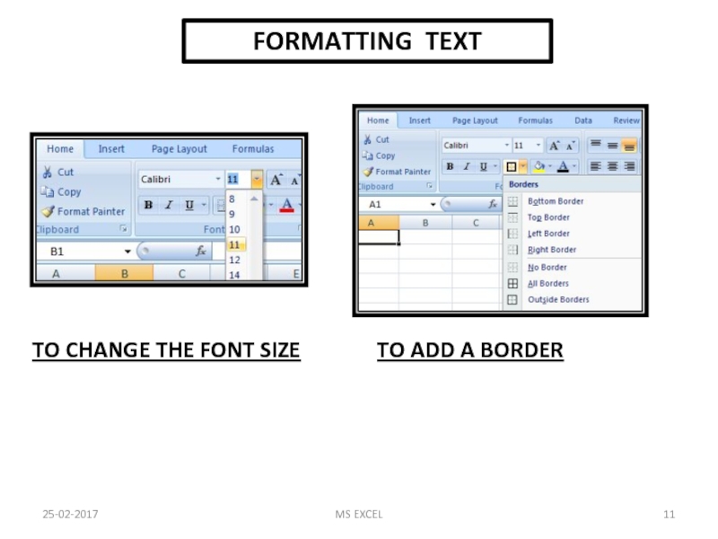
TO CHANGE THE FONT SIZE
TO ADD A BORDER
25-02-2017
MS EXCEL
Слайд 12FORMATTING TEXT
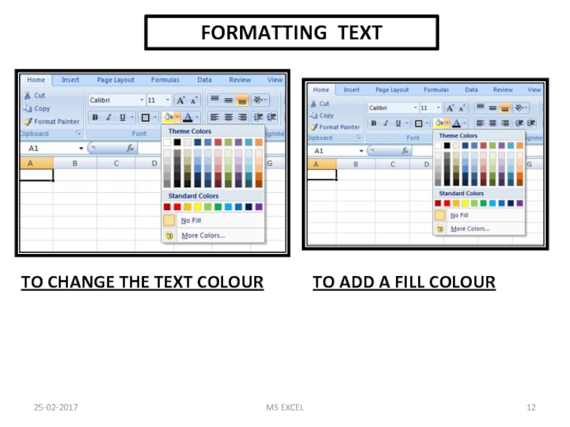
TO CHANGE THE TEXT COLOUR
TO ADD A FILL COLOUR
25-02-2017
MS EXCEL
Слайд 13CONDITIONAL FORMATTING
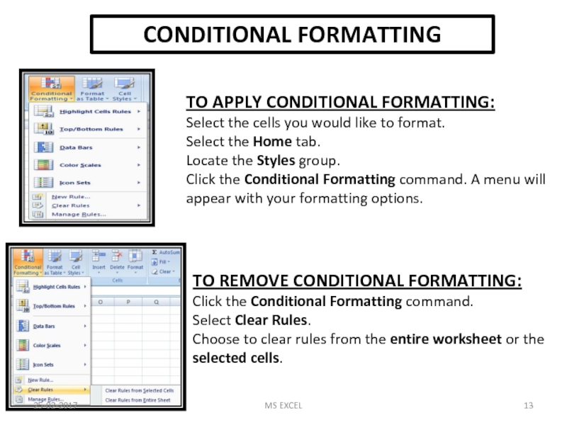
TO APPLY CONDITIONAL FORMATTING:
Select the cells you would like to
format.
Select the Home tab.
Locate the Styles group.
Click the Conditional Formatting command. A menu will appear with your formatting options.
TO REMOVE CONDITIONAL FORMATTING:
Click the Conditional Formatting command.
Select Clear Rules.
Choose to clear rules from the entire worksheet or the selected cells.
25-02-2017
MS EXCEL
Слайд 14CONDITIONAL FORMATTING
TO MANAGE CONDITIONAL FORMATTING:
Click the Conditional Formatting command.
Select Manage Rules
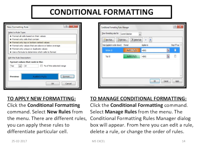
from the menu. The Conditional Formatting Rules Manager dialog box will appear. From here you can edit a rule, delete a rule, or change the order of rules.
TO APPLY NEW FORMATTING:
Click the Conditional Formatting command. Select New Rules from the menu. There are different rules, you can apply these rules to differentiate particular cell.
25-02-2017
MS EXCEL
Слайд 15TO INSERT ROWS & COLUMNS
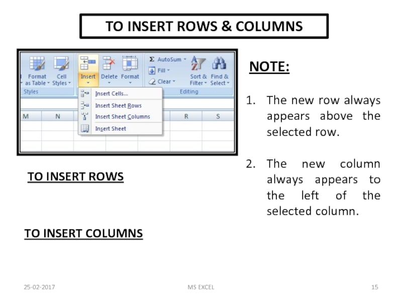
TO INSERT ROWS
TO INSERT COLUMNS
NOTE:
The new
row always appears above the selected row.
The new column always appears to the left of the selected column.
25-02-2017
MS EXCEL
Слайд 1625-02-2017
MS EXCEL
EXCEL AUTOFILL
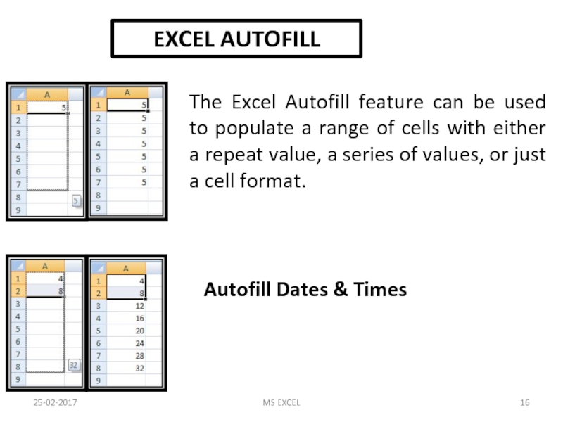
The Excel Autofill feature can be used to populate
a range of cells with either a repeat value, a series of values, or just a cell format.
Autofill Dates & Times
Слайд 17SORTING
TO SORT IN ALPHABETICAL ORDER
TO SORT FROM SMALLEST TO LARGEST
25-02-2017
MS EXCEL

Слайд 18Cell References in Excel
A RELATIVE CELL REFERENCE AS (A1) IS BASED
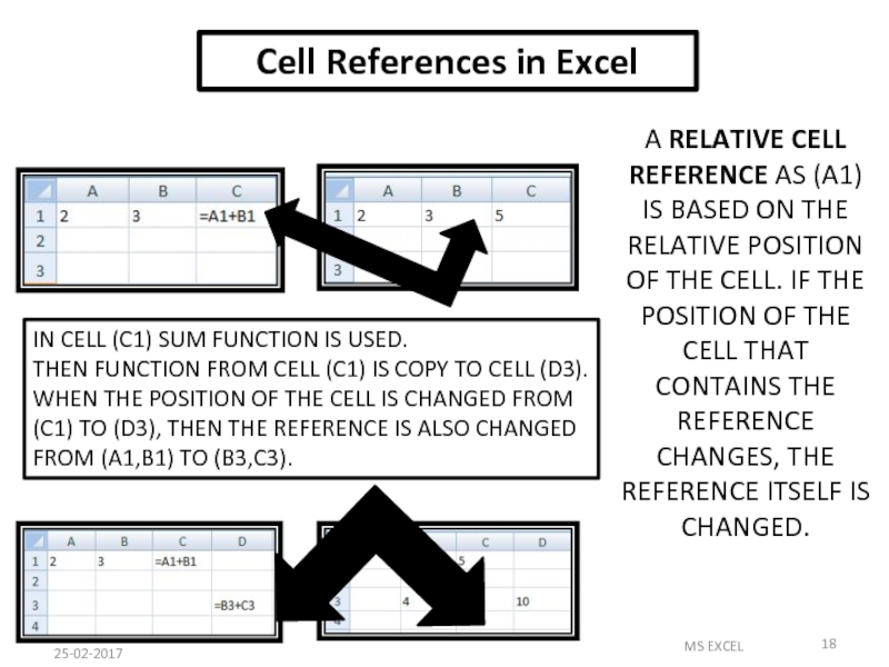
ON THE RELATIVE POSITION OF THE CELL. IF THE POSITION OF THE CELL THAT CONTAINS THE REFERENCE CHANGES, THE REFERENCE ITSELF IS CHANGED.
IN CELL (C1) SUM FUNCTION IS USED.
THEN FUNCTION FROM CELL (C1) IS COPY TO CELL (D3).
WHEN THE POSITION OF THE CELL IS CHANGED FROM (C1) TO (D3), THEN THE REFERENCE IS ALSO CHANGED FROM (A1,B1) TO (B3,C3).
25-02-2017
MS EXCEL
Слайд 19Cell References in Excel
AN ABSOLUTE CELL REFERENCE AS ($A$1) ALWAYS REFERS
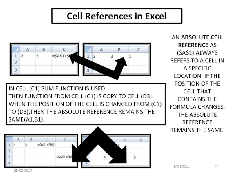
TO A CELL IN A SPECIFIC LOCATION. IF THE POSITION OF THE CELL THAT CONTAINS THE FORMULA CHANGES, THE ABSOLUTE REFERENCE REMAINS THE SAME.
IN CELL (C1) SUM FUNCTION IS USED.
THEN FUNCTION FROM CELL (C1) IS COPY TO CELL (D3).
WHEN THE POSITION OF THE CELL IS CHANGED FROM (C1) TO (D3),THEN THE ABSOLUTE REFERENCE REMAINS THE SAME(A1,B1).
25-02-2017
MS EXCEL
Слайд 20Cell References in Excel
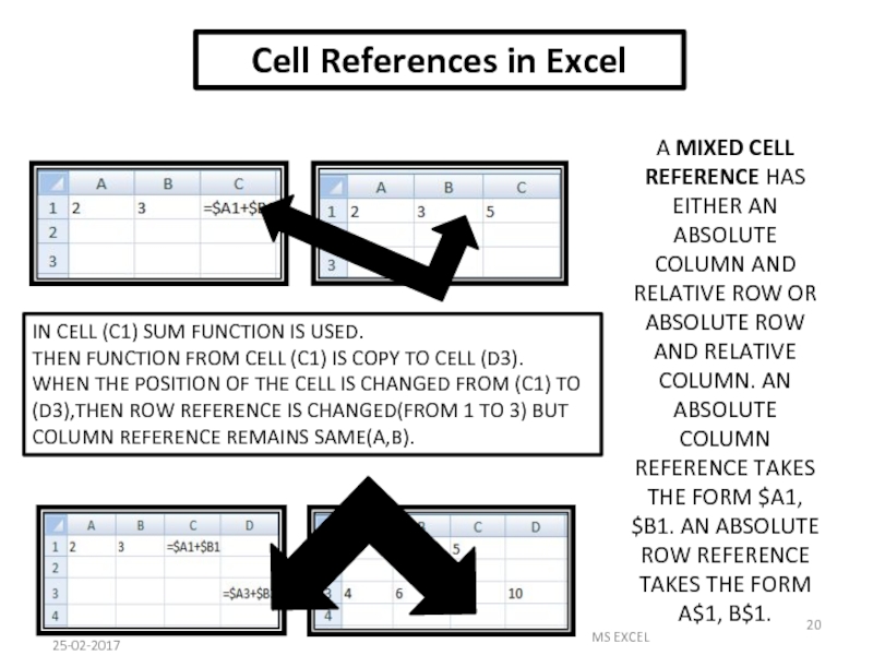
IN CELL (C1) SUM FUNCTION IS USED.
THEN FUNCTION
FROM CELL (C1) IS COPY TO CELL (D3).
WHEN THE POSITION OF THE CELL IS CHANGED FROM (C1) TO (D3),THEN ROW REFERENCE IS CHANGED(FROM 1 TO 3) BUT COLUMN REFERENCE REMAINS SAME(A,B).
A MIXED CELL REFERENCE HAS EITHER AN ABSOLUTE COLUMN AND RELATIVE ROW OR ABSOLUTE ROW AND RELATIVE COLUMN. AN ABSOLUTE COLUMN REFERENCE TAKES THE FORM $A1, $B1. AN ABSOLUTE ROW REFERENCE TAKES THE FORM A$1, B$1.
25-02-2017
MS EXCEL
Слайд 21Relative Cell References
25-02-2017
MS EXCEL
Слайд 22Relative Cell References
25-02-2017
MS EXCEL
Слайд 23Absolute Cell Reference
25-02-2017
MS EXCEL

Слайд 24Absolute Cell Reference
25-02-2017
MS EXCEL

Слайд 25How using cell references with multiple worksheets ?
25-02-2017
MS EXCEL
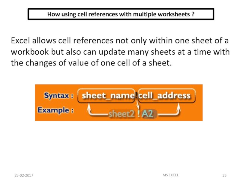
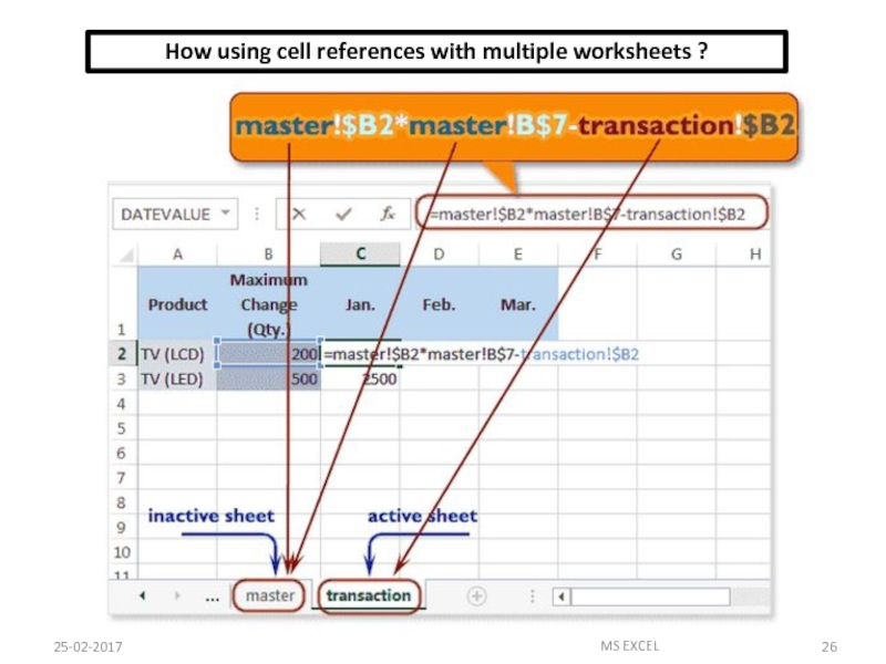
Excel allows
cell references not only within one sheet of a workbook but also can update many sheets at a time with the changes of value of one cell of a sheet.
Слайд 26How using cell references with multiple worksheets ?
25-02-2017
MS EXCEL
Слайд 27FUNCTIONS BASIC
25-02-2017
MS EXCEL
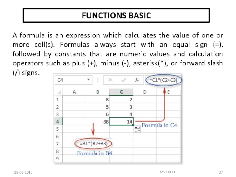
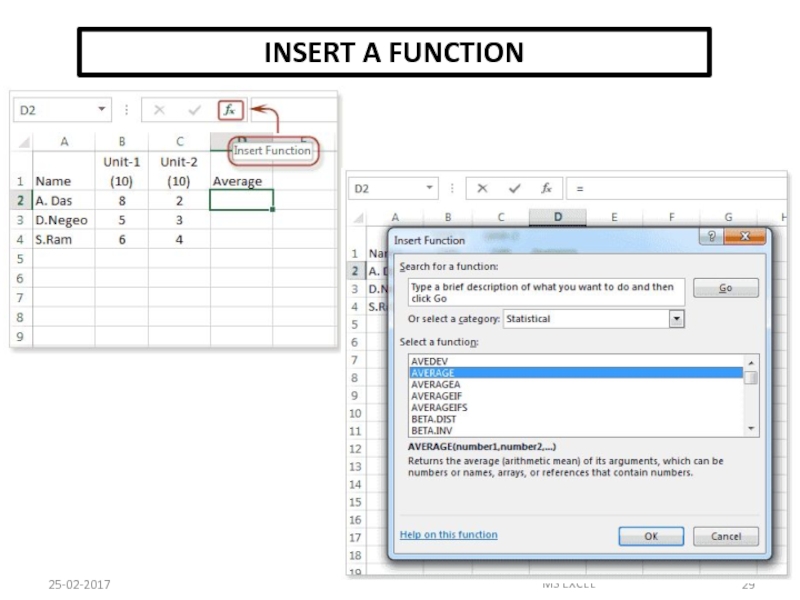
A formula is an expression which calculates the value
of one or more cell(s). Formulas always start with an equal sign (=), followed by constants that are numeric values and calculation operators such as plus (+), minus (-), asterisk(*), or forward slash (/) signs.
Слайд 28INSERT A FUNCTION
25-02-2017
MS EXCEL
Слайд 29INSERT A FUNCTION
25-02-2017
MS EXCEL
Слайд 3025-02-2017
MS EXCEL
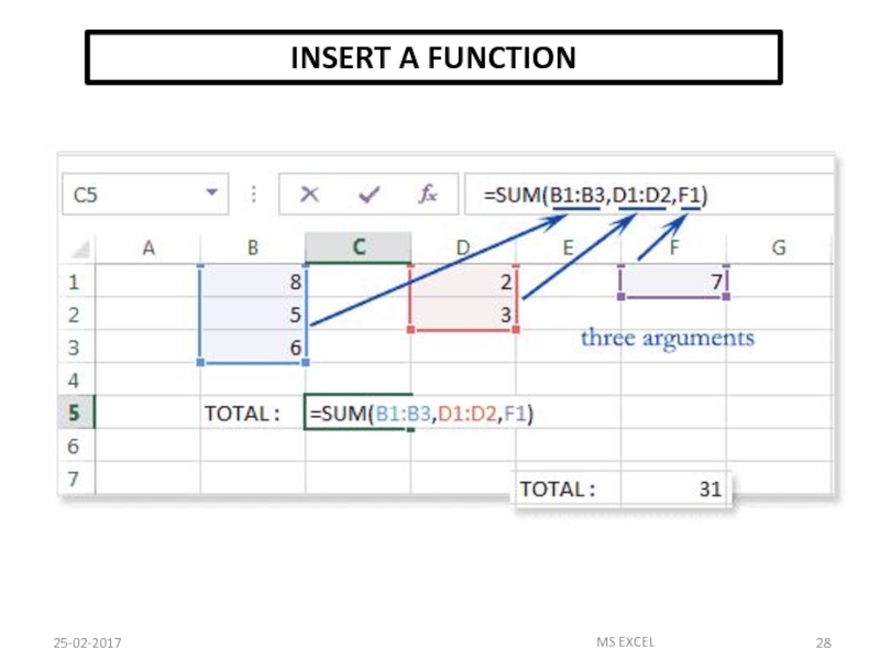
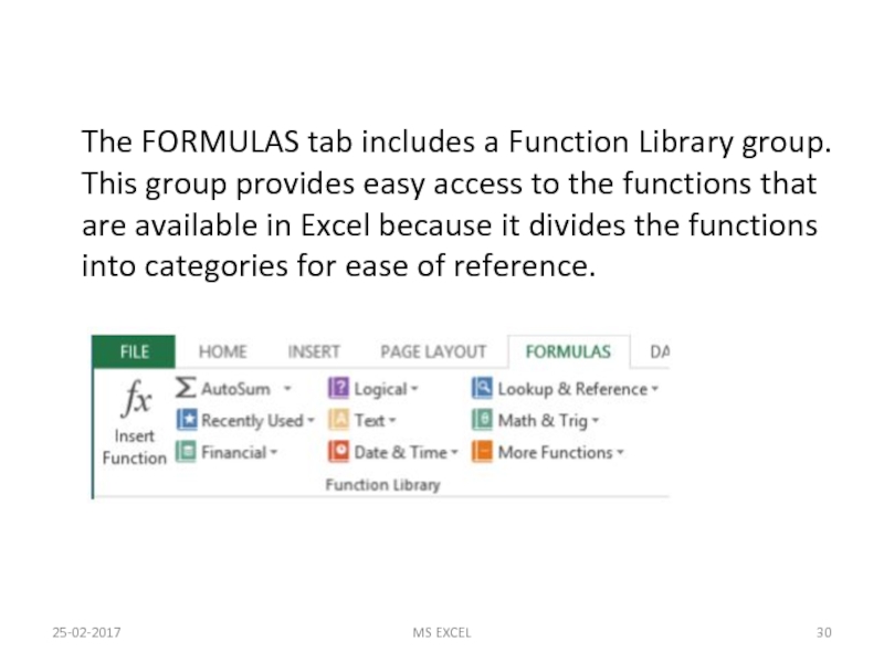
The FORMULAS tab includes a Function Library group. This group
provides easy access to the functions that are available in Excel because it divides the functions into categories for ease of reference.
FUNCTIONS
Слайд 31FUNCTIONS
IF FUNCTION
SYNTAX OF
IF
=IF(LOGICAL TEXT, VALUE IF TRUE, VALUE IF FALSE)
LOGICAL TEXT-
Any value or expression that can be evaluated to TRUE or FALSE.
VALUE IF TRUE-
Value that is returned if logical text is TRUE.
VALUE IF FALSE-
Value that is returned if logical text is FALSE.
25-02-2017
MS EXCEL

Слайд 32FUNCTIONS
SUMIF FUNCTION
SYNTAX OF SUMIF
=SUMIF(RANGE,CRITERIA, [SUM_RANGE])
RANGE-
Range of cells
on which conditions are applied.
CRITERIA-
Condition that defines which cell or cells will be added.
SUM RANGE-
Actual cells to sum.
NOTE:-
If sum range is not used then range is used for sum.
WITHOUT SUM_RANGE
WITH SUM_RANGE
25-02-2017
MS EXCEL
![Introduction to MS EXCEL FUNCTIONSSUMIF FUNCTION SYNTAX OF SUMIF=SUMIF(RANGE,CRITERIA, [SUM_RANGE])RANGE-Range of cells on which FUNCTIONS SUMIF FUNCTION SYNTAX OF SUMIF =SUMIF(RANGE,CRITERIA, [SUM_RANGE]) RANGE- Range of cells on](https://thepresentation.ru/img/tmb/4/382207/a915a8ba2c5ad7713865c1aec08cba64-800x.jpg)
Слайд 33FUNCTIONS
SUMIFS FUNCTION
SYNTAX OF SUMIFS
=SUMIFS(sum_range, criteria_range1, criteria1, [criteria_range2,
criteria2], …)
25-02-2017
MS EXCEL
![Introduction to MS EXCEL FUNCTIONSSUMIFS FUNCTION SYNTAX OF SUMIFS=SUMIFS(sum_range, criteria_range1, criteria1, [criteria_range2, criteria2], …)25-02-2017MS EXCEL FUNCTIONS SUMIFS FUNCTION SYNTAX OF SUMIFS =SUMIFS(sum_range, criteria_range1, criteria1, [criteria_range2, criteria2], …) 25-02-2017](https://thepresentation.ru/img/tmb/4/382207/7bdcad638079085abecb9c1077c22af5-800x.jpg)
Слайд 34COUNT FUNCTIONS
SYNTAX OF FUNCTIONS
1. COUNT(value1, [value2], …)
2. COUNTA(value1, [value2], …)
3.
COUNTBLANK(range)
4. COUNTIF(range, criteria)
5. COUNTIFS(criteria_range1, criteria1, [criteria_range2, criteria2]…)
25-02-2017
MS EXCEL
![Introduction to MS EXCEL COUNT FUNCTIONSSYNTAX OF FUNCTIONS1. COUNT(value1, [value2], …)2. COUNTA(value1, [value2], …) 3. COUNT FUNCTIONS SYNTAX OF FUNCTIONS 1. COUNT(value1, [value2], …) 2. COUNTA(value1, [value2], …) 3. COUNTBLANK(range) 4.](https://thepresentation.ru/img/tmb/4/382207/4224e239de3b12decb6e666b6cad718a-800x.jpg)
Слайд 35Excel Math and Trig Functions
25-02-2017
MS EXCEL
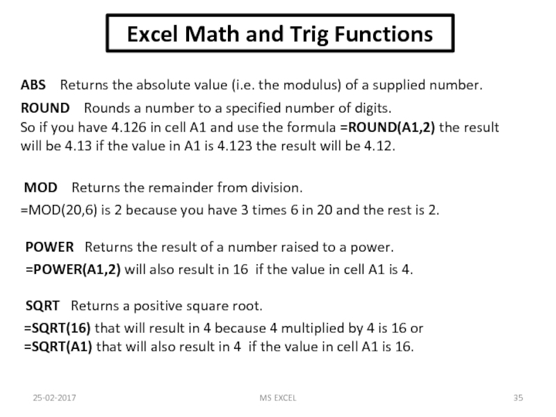
ABS Returns the absolute value
(i.e. the modulus) of a supplied number.
ROUND Rounds a number to a specified number of digits.
So if you have 4.126 in cell A1 and use the formula =ROUND(A1,2) the result will be 4.13 if the value in A1 is 4.123 the result will be 4.12.
MOD Returns the remainder from division.
=MOD(20,6) is 2 because you have 3 times 6 in 20 and the rest is 2.
POWER Returns the result of a number raised to a power.
=POWER(A1,2) will also result in 16 if the value in cell A1 is 4.
SQRT Returns a positive square root.
=SQRT(16) that will result in 4 because 4 multiplied by 4 is 16 or
=SQRT(A1) that will also result in 4 if the value in cell A1 is 16.
Слайд 36Excel Math and Trig Functions
25-02-2017
MS EXCEL
Слайд 3725-02-2017
MS EXCEL
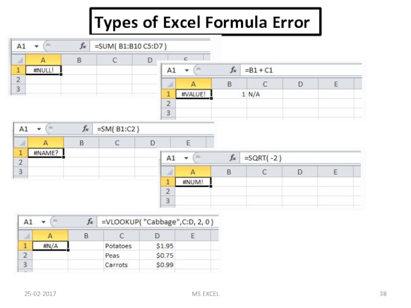
Types of Excel Formula Error
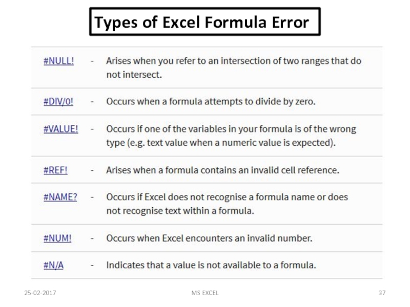
Слайд 3825-02-2017
MS EXCEL
Types of Excel Formula Error
