

OFFSET MATCH MATCH is the final lookup combination I’ll cover among the lookup formula options you have available to you in Excel. Of all the different lookup options you have to do a two-way lookup, INDEX MATCH MATCH is still probably your best bet and the approach I would generally recommend. However, OFFSET MATCH MATCH is a viable alternative. In some ways, using the OFFSET function to find a lookup value is more intuitive because it is very similar to moving a piece around a chess board. Additionally, some people are more familiar with the OFFSET function than they are with INDEX; in that situation, it may make sense to go with OFFSET MATCH MATCH as your lookup formula.
Objective and When to Use
There’s only one simple requirement for using OFFSET MATCH MATCH: the need to perform a matrix style lookup. To put it in simple terms:
The data table you use must have lookup values on both the left hand side as well as the top header row
See the table below for a simple example, with lookup values for country on the left hand side and lookup values for year in the top header row.

Now, when comparing OFFSET MATCH MATCH to INDEX MATCH MATCH, the only real difference is the foundational formula.
INDEX requires you to:
- Define a particular reference array
- Then Excel asks you to tell it where to move within that defined space
In contrast, OFFSET asks you to:
- Designate a starting point
- Then Excel asks you to tell it how to move away from that starting point
They’ll both essentially end up with the same result. OFFSET MATCH MATCH just provides you a slightly different way of getting there. As the post picture suggests, using OFFSET MATCH MATCH is like directing a chess piece a specified number of steps away from a particular space on the board.
The Syntax
= OFFSET ( MATCH ( lookup_value , lookup_array , 0 ) , MATCH ( lookup_value , lookup_array , 0 ) )
The overall syntax for the OFFSET MATCH MATCH formula combination is fairly intuitive. You have OFFSET as your primary formula with two MATCH formulas designating the vertical and horizontal offset. We’ll go into detail with both formulas below.
The OFFSET Formula
= OFFSET ( reference , rows , cols , [height] , [width] )
The OFFSET formula asks you to specify a starting reference point, and then designate how many cells you want to move vertically (rows) and horizontally (columns) away from that intial reference. OFFSET then pulls the value you land on after making those moves.
The height and width syntax inputs at the end are optional and only used if you want to return a range larger than a single cell. For example, if you wanted Excel to return a range cells that’s 3 x 4 cells large, then you would input 4 and 3 respectively for those syntax inputs.
For this tutorial, we’ll only need to return a single cell, so we will not be using those syntax inputs.
The MATCH Formula
= MATCH ( lookup_value , lookup_array , 0 )
The MATCH formula asks you to specify a value within a range and returns the position of that value within that range. For example, using the table shown above, if I selected 2012 as my lookup value and selected the entire top row as my lookup array, the MATCH formula would return the number “2” because 2012 is the second value in the array I selected. Also note that at the very end of the syntax, you need to put in a “0” as the last argument to direct the MATCH formula to perform an exact match lookup.
Putting it All Together
Below is a simplified version of the syntax that you can use for reference when you want to remember the formula combination:
= OFFSET ( starting point , MATCH ( vertical lookup value, left hand lookup column excluding starting point , 0 ) , MATCH ( horizontal lookup value , top header row excluding starting point , 0 ) )
Goal: Assume we want to find the Revenue amount for Brazil in the year 2014
Step 1: Start writing your OFFSET formula and select your starting reference point, which will be the upper left hand corner of your table. In this case it’s the cell containing the word “Country”.

Step 2: Start your MATCH formula and select your vertical lookup value, in this case, the country China

Step 3: Identify your vertical lookup array. This is your vertical column EXCLUDING the cell you originally selected as your starting point. In this case, it’s the cells with country names, highlighted in purple below.

Step 4: Close out your MATCH formula by inputting “0” for exact match.

Step 5: Start your MATCH formula and select your horizontal lookup value, in this case, the year 2015

Step 6: Identify your horizontal lookup array. This is your top row EXCLUDING the cell you originally selected as your starting point. In this case, it’s the cells with year values, highlighted in magenta below.

Please Note: Make sure that you do not overlap your MATCH selection arrays with your starting point. Note that in all of the selections above, none of them overlap or cross one another. This is because the MATCH formula informs your OFFSET formula regarding how many cells to move AWAY from the starting point. If you overlap the selection, it will make it move an extra step away from your target. This is probably the most common mistake made when using OFFSET MATCH MATCH. The lack of overlap is also one key difference that this formula combination has with INDEX MATCH MATCH.
Step 7: Close out your MATCH formula by inputting “0” for exact match

Step 8: Add one final parenthesis to close out the OFFSET MATCH MATCH combination formula

What Excel Does
The first thing Excel will do is process your MATCH formulas. Excel will determine the relative position of your lookup values within the lookup arrays you’ve selected. In this scenario, China and 2015 are both in the 4th position in their relative arrays. Excel now knows how many cells to move down and how many cells to move right.

Starting from your original starting cell of “Country”, Excel will move 4 cells down and 4 cells right. The resulting value for the entire formula combination is whatever cell Excel finally lands on, which in this case is $2,251.67.

Summary
The primary benefit of using OFFSET MATCH MATCH is that it is intuitive and that many people are familiar with the OFFSET formula. For those reasons, it’s important to at least consider this formula combination among your lookup options.
The VLOOKUP, HLOOKUP and INDEX-MATCH are famous and common ways to lookup a values in Excel table. But these are not the only ways to lookup values in Excel. In this article, we will learn how to use the OFFSET function along with the MATCH function in Excel. Yes you read it right, we will use the infamous OFFSET function of Excel to lookup a certain value in a Excel Table.
Generic Formula,
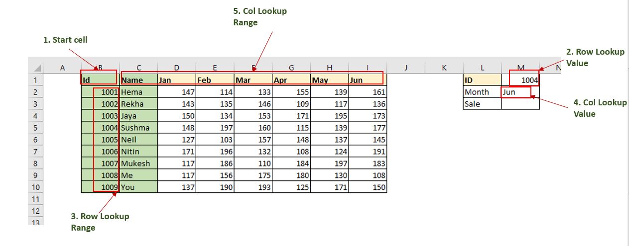
=OFFSET(StartCell,MATCH(RowLookupValue,RowLookupRange,0),MATCH(ColLookupValue,ColLookupRange,0))
Read this carefully:
StartCell: This is the starting cell of lookup Table. Let’s say if you want to lookup in range A2:A10, then the StartCell will be A1.
RowLookupValue: This is the lookup value that you want to find in rows below the StartCell.
RowLookupRange: This is the range in which you want to lookup the RowLookupValue. It is the range below StartCell (A2:A10).
ColLookupValue: This is the lookup value that you want to find in columns (headers).
ColLookupRange: This is the range in which you want to lookup the ColLookupValue. It is the range on the right hand side of StartCell (like B1:D1).
So, enough of the theory. Let’s get started with an example.
Example: Lookup Sales Using OFFSET and MATCH function From Excel Table
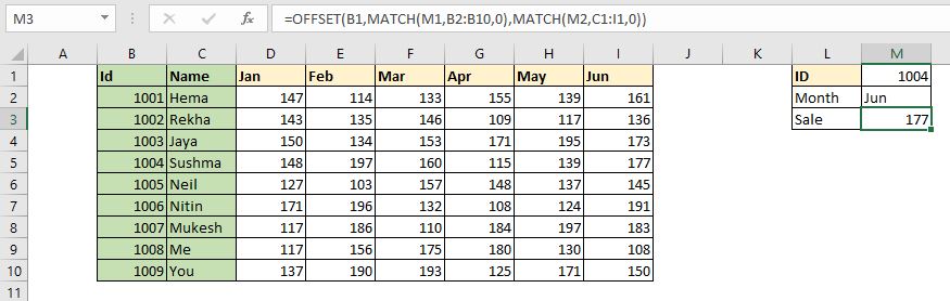
Here we have a sample table of sales done by different employees in different months.
Now our boss is asking us to give the sales done by Id 1004 in the Jun month. There are many ways to do it but since we are learning about the OFFSET-MATCH formula, we will use them to lookup the desired value.
We already have the generic formula above. We just need to identify these variables in this table.
StartCell is B1 here. RowLookupValue is M1. RowLookupRange is B2:B1o (range below the startcell).
ColLookupValue is in M2 cell. ColLookupRange is C1:I1 (Header Range on the right of the StartCell) .
We have identified all the variables. Let’s put them into an Excel Formula.
Write this formula in Cell M3 and hit the enter button.
As you hit the enter button, you get the result promptly. The sale done ID 1004 in Jun Month is 177.
How does it work?
The OFFSET function’s work is to move away from the given starting cell to given row and columns and then return value from that cell. For example, If I write OFFSET(B1,1,1), the OFFSET function will go to cell C2 (1 cell down, 1 cell to right) and returns it value.
Here, We have formula OFFSET(B1,MATCH(M1,B2:B10,0),MATCH(M2,C1:I1,0)).
The first MATCH function returns the index of M1 (1004) in range B2:B10, which is 4. Now the formula is, OFFSET(B1,4,MATCH(M2,C1:I1,0)).
Next MATCH function returns the index of M2 (‘Jun’) in range C1:I1, which i 7. Now the formula is OFFSET(B1,4,7).
Now the OFFSET function simply moves 4 cells down to the cell B1 which takes it to B5. Then the OFFSET function moves to 7 left to B5, which takes it to I5. That is it. The OFFSET function returns value from cell I5 which 177.
Advantages of this lookup technique?
This is fast. The sole advantage of this method is that it is faster than the other methods. The same thing can be done using the INDEX-MATCH function, or VLOOKUP function. But it is good to know some alternatives. It may come handy some day.
So yeah guys, this is how you can use the OFFSET and MATCH function to LOOKUP values in Excel Tables. I hope it was explanatory enough. If you have any doubts regarding this article or any other excel/VBA related topic, ask me in the comments section below.
Related Articles:
Use INDEX and MATCH to Lookup Value: The INDEX-MATCH formula is used to lookup dynamically and precisely a value in given table. This is an alternative to the VLOOKUP function and it overcomes the shortcomings of the VLOOKUP function.
Sum by OFFSET groups in Rows and Columns: The OFFSET function can be used to sum group of cells dynamically. These groups can be anywhere in the sheet.
How to Retrieve Every Nth Value in a Range in Excel: Using the OFFSET function of Excel we can retrieve values from alternating rows or columns. This formula takes help of the ROW function to alternate through rows and COLUMN function to alternate in columns.
How to use OFFSET Function in Excel: The OFFSET function is a powerful Excel function that is underrated by many users. But experts know the power of the OFFSET function and how can we use this function to do some magical tasks in Excel formula. Here are the basics of the OFFSET function.
Popular Articles:
50 Excel Shortcuts to Increase Your Productivity | Get faster at your task. These 50 shortcuts will make you work even faster on Excel.
How to use Excel VLOOKUP Function| This is one of the most used and popular functions of excel that is used to lookup value from different ranges and sheets.
How to use the Excel COUNTIF Function| Count values with conditions using this amazing function. You don’t need to filter your data to count specific values. The COUNTIF function is essential to prepare your dashboard.
How to Use SUMIF Function in Excel | This is another dashboard essential function. This helps you sum up values on specific conditions.
I’m using match() to locate a cell with a specific value in column A.
=MATCH("Sales",A:A,0)
This returns the row value 40 for example.
I want to then use this value with OFFSET() like so:
=OFFSET(MATCH("Sales",A:A,0),1,1)
So if my match() returned A40, offset() would then give me the value of B41. Unfortunately, this does not work. What can I do to achieve this?
asked Jan 4, 2017 at 18:31
![]()
1
Use INDEX instead:
=INDEX(B:B,MATCH("Sales",A:A,0)+1)
OFFSET is volatile and should only be used when no other option is available.
answered Jan 4, 2017 at 18:32
![]()
Scott CranerScott Craner
146k9 gold badges47 silver badges80 bronze badges
Related Links: 1. Excel VLOOKP Function, with examples. 2. Left Lookup with VLookup Excel function 3. Vlookup Multiple Values — Return MULTIPLE corresponding values for ONE Lookup Value. 4. Case Sensitive Vlookup; Finding the 1st, 2nd, nth or last occurrence of the Lookup Value.
 Left Lookup, with Index & Match functions
=INDEX($A$1:$D$10, MATCH(450,$B$1:$B$10, 0),1) [Formula]
The formula does a loookup of «450» in column B and returns corresponding value in column A, which is «Laurel». (Refer Table 1)
Returns the value (Laurel) in an array ($A$1:$D$10), at row_num 5 (5 is returned by the below MATCH function) and column_num 1 (ie. column A).
=MATCH(450, $B$1:$B$10, 0) [Formula Break]
This part of the formula returns the value 5, which is the relative position of Lookup_value (ie. 450) in the lookup_array ($B$1:$B$10).
——————————————————————————————————
Left Lookup, with Index & Match functions
=INDEX($A$1:$D$10, MATCH(450,$B$1:$B$10, 0),1) [Formula]
The formula does a loookup of «450» in column B and returns corresponding value in column A, which is «Laurel». (Refer Table 1)
Returns the value (Laurel) in an array ($A$1:$D$10), at row_num 5 (5 is returned by the below MATCH function) and column_num 1 (ie. column A).
=MATCH(450, $B$1:$B$10, 0) [Formula Break]
This part of the formula returns the value 5, which is the relative position of Lookup_value (ie. 450) in the lookup_array ($B$1:$B$10).
——————————————————————————————————
Left Lookup, with Offset & Match functions =OFFSET($A$1:$D$10, MATCH(C4, OFFSET($A$1:$D$10, 0,2, ROWS($A$1:$D$10), 1),0)-1, 0,1,1) [Formula] The formula does a loookup of C4 in column C and returns corresponding value in column A, which is «Juliet». (Refer Table 2) The value of 3 (returned from MATCH function below), is used for «rows» in this OFFSET formula. Formula Offsets 3 rows down from A1, in same column A (cols = 0), single cell (height, width being 1) ie. A4, and returns value in cell A4, which is «Juliet». =ROWS($A$1:$D$10) [Formula Break] This part of the formula returns the value 10, which is the number of rows in a reference or array. Syntax: ROWS(array). =OFFSET($A$1:$D$10, 0,2, ROWS($A$1:$D$10), 1) [Formula Break] This part of the formula returns one column (width = 1) with 10 rows (height = 10), starting 2 columns (cols = 2) to the right of column A (viz column C). The returned column C1:C10, is the one in which Lookup value C4 is present. =MATCH(C4, OFFSET($A$1:$D$10, 0,2, ROWS($A$1:$D$10),1), 0)-1 [Formula Break] Match Function returns the value 3, which is the position of C4 in Column C1:C10 (4). We deduct 1 from the match result of 4, for use in OFFSET function (4 minus 1 = 3).
In Excel, a dynamic range is a reference (or a formula you use to create a reference) that may change based on user input or the results of another cell or function. It is more than just a fixed group of cells like $A1:$A100. I use dynamic ranges mostly for customizable drop-down lists. To avoid showing a bunch of blanks in the list, I use a formula to reference a range that extends to the last value in a column. The image below shows 4 different formulas that reference the range A2:A9 and can expand to include more rows if the user adds more categories to the list.
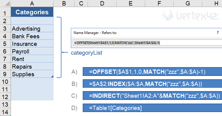
When we talk about a dynamic named range, we’re talking about using the Name Manager (via the Formula tab) to define a name for the formula, such as categoryList. We can then use that Name in other formulas or as the Source for drop-down lists.
This article isn’t about the awesome advantages of using Excel Names, though there are many. Instead, it is about the many different formulas you can use to create the dynamic named ranges.
To see these examples in action, download the Excel file below.
Download the Example File (DynamicRanges.xlsx)
Do you have a Dynamic Named Range challenge you need to solve? If you can’t figure it out after reading this article, go ahead and ask your question by commenting below.
This Page (contents):
- A) The OFFSET Function
- B) The INDEX Function for a Non-Volatile Dynamic Range
- C) The INDIRECT Function
- D) Structured References with Excel Tables
- E) The CHOOSE and IF Functions
- Find the Position of the LAST Value in the Column
- Bonus: Create a Dynamic Print Area
- No Dynamic Named Ranges in Google Sheets
Watch the Video
A) The OFFSET Function
The most common function used to create a dynamic named range is probably the OFFSET function. It allows you to define a range with a specific number of rows and columns, starting from a reference cell. The syntax for the OFFSET function is:
=OFFSET(reference,offset_rows,offset_cols,[height],[width])
The offset_rows and offset_cols values tell the function where you want the upper-left cell of your range to be, relative to the reference cell. The height and width values tell the function how many rows and columns you want to include in your range.
A Basic Customizable List
In the meal planner template, I have a list of meals that I use as the Source for many different drop-down lists. I want to allow the user to edit and add to the list, so the dynamic named range used by the drop-down needs to extend to the last value in the list. I could define the range as $A:$A (the entire column) or $A1:$A1000 (assuming they won’t add more than 1000 items to the list), but then I’d end up with a bunch of blank cells at the end of my drop-down list.
Using the OFFSET function, I define a range that starts at cell $A$1 and ends at the cell containing the last value in the column. If the last value in the column was on row 15, the formula for the named range would be:
=OFFSET($A$1,0,0,15,1)
To make this formula dynamic, I’ll use a formula or reference in place of the height value (15) to specify how many rows I want the range to include. I expect only text values in this list, so I’ll use the MATCH function to find the last text value in the column like this:
=OFFSET($A$1,0,0,MATCH("zzzz",$A:$A),1)
There are many formulas you can use to determine the height or width of the range, such as COUNTA, COUNT, VLOOKUP, LOOKUP, MATCH or various array formulas. What formula you use may depend on whether you expect there to be blank cells in the list, error values (like #N/A or #DIV/0!), or data of different types (text or numeric or both), and whether calculation speed is an issue.
Later in this article I’ll talk more about the various formulas for finding the last value in the range. For now, we’ll continue using MATCH.
A Robust Dynamic Range
When you allow a user to edit a list, they may end up deleting the first row in the list, or they might insert a row above the first row in the list (between the label row and the first item). To create a formula that works in spite of these actions by the user, I like to use a label for the reference and include the label in the range, as shown in the following examples.
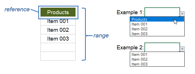
Example 1: Include the label in the list
=OFFSET(reference,0,0,MATCH("zzz",range),1)
Example 2: Exclude the label from the list
=OFFSET(reference,1,0,MATCH("zzz",range)-1,1)
Notice in the second example that reference and range have not changed. To exclude the label from the list, we are using an offset of 1 row and subtracting one row from the number returned by the MATCH function.
B) The INDEX Function for a Non-Volatile Dynamic Range
A volatile function within a cell or named range is recalculated every time any cell in the worksheet recalculates (instead of just when one of the function’s arguments changes). Also, any formula that depends on a cell containing a volatile function is also recalculated. If you have a large file with thousands of inefficient formulas that reference a cell containing a volatile function, Excel may seem to take forever to recalculate. OFFSET is a volatile function. INDEX is not, so some people prefer to use INDEX for dynamic ranges.
The INDEX function can return the reference to a range or cell instead of just the value. That means that just like OFFSET, you can use INDEX in many places where Excel is expecting a cell reference. For example, to create the range A1:A4 you can use INDEX(A:A,1):INDEX(A:A,4).
We can use INDEX to create the same dynamic ranges shown in the OFFSET examples:
Example 1: Include the label in the list
=INDEX(range,1):INDEX(range,MATCH("zzz",range))
Example 2: Exclude the label from the list
=INDEX(range,2):INDEX(range,MATCH("zzz",range))
To exclude the label (the first cell in the range), the only change we needed to make was the «2» in INDEX(range,2). Using INDEX(range,1) and INDEX(range,2) instead of just a cell reference makes the formula more robust. It prevents the problem of having the reference changed to #REF! if the reference row gets deleted.
NOTEWhen using INDEX, the formulas cannot be entered directly as the Source for a drop-down list. But, if you create the formula as a dynamic named range, you can use the name as the Source for the drop-down list.
By the way, I learned about using the INDEX function to make a non-volatile dynamic range from Mynda Treacy at MyOnlineTrainingHub.com and Debra Dalgleish at Contextures.com.
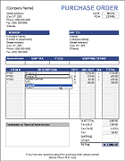 Purchase Order with Price List
See Dynamic Named Ranges in action. This template uses multiple customizable lists for selecting items descriptions, vendor and ship to addresses, and other options. The item description list uses the OFFSET formula and the other lists use the INDEX formula.
C) The INDIRECT Function
The INDIRECT function is another awesome function for creating dynamic ranges. It is also a volatile function, but like I mentioned above, that might not matter. The INDIRECT function lets you define a reference from a text string, and you can use concatenation to create the text string, like this:
=INDIRECT("Sheet1!A1:A"&row_num)
In the example shown at the top of this post, to create the reference «Sheet1!A2:A9» we replace row_num with MATCH(«zzz»,$A:$A) to return the row number of the last text value.
Important: When using INDIRECT to reference a range on a different worksheet, don’t forget to include the worksheet name in the string. When you enter a reference in the Refers To field via the Name Manager, Excel will automatically change $A:$A to «Sheet1!$A:$A» but it won’t know how to change your text string. This is one of the cons to using INDIRECT because if you change the name of the worksheet, you’ll need to remember to update your INDIRECT formula.
D) Structured References with Excel Tables
Beginning with Excel 2007, Microsoft introduced a new way to work with data in what are called Excel Tables, not to be confused with Data Tables, or other generic uses of the term table (yes, it is confusing).
If you use an official «Excel Table,» you can use a type of reference known as a structured reference. The structured reference uses the table name and the column labels like this:
=Table1[Categories]
You don’t need to know how to type the correct structured reference. While you are entering a formula, if you select the column in the Table, Excel will automatically change your reference to the structured reference.
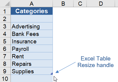
The reason these types of references can be considered dynamic is because of the unique way that table references behave when you expand or contract the table. Meaning, if you extend the table down by dragging the resize handle in the lower-right corner of the table, the reference =Table1[Categories] will automatically include the new rows.
So, instead of using an OFFSET formula to extend a range to the last value in a customizable list, we can let the user change the size of the list using the drag handle. Of course, this requires the user to know how to use Tables and the drag handle. That is one of the reasons I don’t often use this technique in my templates (that, and lack of compatibility with OpenOffice and Google Sheets).
E) The CHOOSE and IF Functions
Although I don’t use the CHOOSE function or nested IF formulas to create lists of variable length, they are pretty powerful functions for creating other types of dynamic ranges. For example, the two formulas below both return a different range (range_1, range_2 or range_3) based on a given number:
=CHOOSE(number,range_1,range_2,range_3,...)
=IF(number=1,range_1,IF(number=2,range_2,IF(number=3,range_3)))
The CHOOSE function is basically a shortcut for the nested IF formula in this case. When possible, I prefer using CHOOSE over nested IF formulas (if only to avoid having a million closing parentheses at the end of the formula ))))))))))).
See CHOOSE in action: My article «Create a Drop Down List in Excel» shows an example using CHOOSE to create a dependent drop down list.
Find the Position of the LAST Value in the Column
When using a dynamic named range for lists of variable length, we need to know how to find the numeric position of the last value in the column. In the examples above we used MATCH(«zzz»,range) for text values, but for numeric data or a combination of text and numeric data we may need to use something different. The formulas below cover all the scenarios I’ve come across.
The following image will be used for the example. It shows the reference and range and the position numbers of the values in the range.

1. Find the Position of the Last Numeric Value
The following formulas will allow the range to include blanks, error values, and text values, but the formulas will only return the position of the last numeric value. The result would be 4 in the example above.
=MATCH(1E+100,range,1)
=LOOKUP(42,1/ISNUMBER(range),ROW(range)-ROW(reference)+1)
See my article about VLOOKUP and INDEX-MATCH for a more detailed explanation of these MATCH and LOOKUP formulas. LOOKUP does not behave the same way in OpenOffice and Google Sheets. So, for maximum compatibility, I still prefer to use MATCH.
The value 9.99999999999999E+307 could be used for the MATCH function because it is the largest numeric value that can be stored in a cell, but that is kind of overkill. I prefer to use something more concise like 1E+100 or 10^100 (a googol).
2. Find the Position of the Last Text Value
The following formulas will allow the range to include blanks, error values, and numeric values, but the formulas will only return the position of the last text value (row 5 in the example above).
=MATCH("zzzz",range,1)
=LOOKUP(42,1/ISTEXT(range),ROW(range)-ROW(reference)+1)
Note: Using «zzzz» for the lookup value is not fool proof. The Greek, Cyrillic, Hebrew, and Arabic Unicode characters (and possibly other Unicode characters) come after z in the sort order. You might try using a high-value unicode symbol such as 🗿 if you expect the list to contain symbols.
3. Find the Position of the Last Non-Blank Value
When we want to return the last non-blank value, we can use the largest position returned by the two MATCH formulas listed above, or we can use the LOOKUP formula.
=MAX(MATCH(9E+307,range),MATCH("🗿",range))
=LOOKUP(42, 1/NOT(ISBLANK(range)), ROW(range)-ROW(reference)+1 )
Note that the empty string «» is not blank. It is treated as a text value.
A cell containing a formula is not blank, even if the formula returns an empty string. So, use the next method if you want to find the last non-empty value when you are using formulas that might return an empty string.
4. Find the Position of the Last Non-Empty Value «»
In many practical applications (like loan calculators), we may not necessarily want to find the last non-blank cell ( meaning no values or formulas), but instead may want to find the last non-empty cell.
If we define «empty» as the empty string «», then we can return the last non-empty value using the formula below. This might look like an array formula, but it isn’t, thanks to the way LOOKUP works (See this article on exceljet.net).
=LOOKUP(42, 1/(range<>""), ROW(range)-ROW(reference)+1 )
As I mentioned before, LOOKUP does not work the same way in OpenOffice and Google Sheets, but SUMPRODUCT provides a good solution.
=SUMPRODUCT(MAX((range<>"")*(ROW(range)-ROW(reference)+1)))
The SUMPRODUCT function allows you to avoid entering the formula as an array formula (not having to use Ctrl+Shift+Enter). Inside the SUMPRODUCT function, we are multiplying the boolean (FALSE=0 or TRUE=1) result for the (range<>»») comparison by the relative row number, so that the maximum result is the row number of the last blank cell.
Bonus: Create a Dynamic Print Area
When you create a print area in Excel via Page Layout > Print Area > Set Print Area, Excel actually creates a special named range called Print_Area. You can then go to Formulas > Name Manager and edit that named range to use a formula like this:
=OFFSET(start_cell,0,0,rows,columns)
This is a technique I use in some financial templates like the Home Mortgage Calculator to limit the print area based on the length of the payment schedule.
The catch: If you edit the Page Layout (margins, scaling, etc.), the Print_Area reference is changed to a regular reference. I’m not sure why the formula is removed, but this is basically a bug in Excel that has yet to be resolved. To avoid recreating the formula, I typically copy the formula and paste it into a text editor so that I can easily recreate the dynamic print area after I’m done making changes to the page layout.
No Dynamic Named Ranges in Google Sheets
Perhaps things will change in the future, but as of my last update (Sep 28, 2017), you cannot create named formulas using the Named Ranges feature in Google Sheets. This means that although you can use a Named Range for a drop-down list, you can’t create a Dynamic Named Range using a formula in Google Sheets.
Ben Collins shows how you can use a cell to create a text string like «A1:A»&row_num, name the cell, and then use INDIRECT(theName) to get some of the function of a dynamic named range. Unfortunately, that still doesn’t work for drop-down lists, because you can’t use INDIRECT(theCell) as the Range for a drop-down list.
References Related to Dynamic Named Ranges
- Dynamic Named Ranges at ozgrid.com — I think Dave Hawley’s site is the first place I saw the term «dynamic named range» used. Now, you can find articles on the subject at most Excel help sites.
- Using structured references with Excel tables at support.office.com
- Excel Named Ranges at contextures.com — A great article by Debra Dalgleish about how to create and use named ranges in Excel.