Excel обязательно are you - Word и Excel - помощь в работе с программами

Содержание

Использование ЕСЛИ с функциями И, ИЛИ и НЕ
Примеры
Использование операторов И, ИЛИ и НЕ с условным форматированием
Дополнительные сведения
См. также
Using IF with AND, OR and NOT functions
Examples
Using AND, OR and NOT with Conditional Formatting
Need more help?
See also
Excel Wildcard Characters – What are these and How to Best Use it
Excel Wildcard Characters – An Introduction
Excel Wildcard Characters – Examples
#1 Filter Data using Excel Wildcard Characters
#2 Partial Lookup Using Wildcard Characters & VLOOKUP
3. Find and Replace Partial Matches
4. Count Non-blank Cells that Contain Text

Использование ЕСЛИ с функциями И, ИЛИ и НЕ

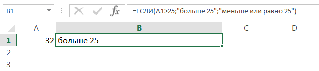
Функция ЕСЛИ позволяет выполнять логические сравнения значений и ожидаемых результатов. Она проверяет условие и в зависимости от его истинности возвращает результат.

=ЕСЛИ(это истинно, то сделать это, в противном случае сделать что-то еще)

Но что делать, если необходимо проверить несколько условий, где, допустим, все условия должны иметь значение ИСТИНА или ЛОЖЬ ( И), только одно условие должно иметь такое значение ( ИЛИ) или вы хотите убедиться, что данные НЕ соответствуют условию? Эти три функции можно использовать самостоятельно, но они намного чаще встречаются в сочетании с функцией ЕСЛИ.

Используйте функцию ЕСЛИ вместе с функциями И, ИЛИ и НЕ, чтобы оценивать несколько условий.

ЕСЛИ(И()): ЕСЛИ(И(лог_выражение1; [лог_выражение2]; …), значение_если_истина; [значение_если_ложь]))

ЕСЛИ(ИЛИ()): ЕСЛИ(ИЛИ(лог_выражение1; [лог_выражение2]; …), значение_если_истина; [значение_если_ложь]))

ЕСЛИ(НЕ()): ЕСЛИ(НЕ(лог_выражение1), значение_если_истина; [значение_если_ложь]))

Условие, которое нужно проверить.

Значение, которое должно возвращаться, если лог_выражение имеет значение ИСТИНА.

Значение, которое должно возвращаться, если лог_выражение имеет значение ЛОЖЬ.

Общие сведения об использовании этих функций по отдельности см. в следующих статьях: И, ИЛИ, НЕ. При сочетании с оператором ЕСЛИ они расшифровываются следующим образом:

И: =ЕСЛИ(И(условие; другое условие); значение, если ИСТИНА; значение, если ЛОЖЬ)

ИЛИ: =ЕСЛИ(ИЛИ(условие; другое условие); значение, если ИСТИНА; значение, если ЛОЖЬ)

НЕ: =ЕСЛИ(НЕ(условие); значение, если ИСТИНА; значение, если ЛОЖЬ)

Примеры

Ниже приведены примеры распространенных случаев использования вложенных операторов ЕСЛИ(И()), ЕСЛИ(ИЛИ()) и ЕСЛИ(НЕ()). Функции И и ИЛИ поддерживают до 255 отдельных условий, но рекомендуется использовать только несколько условий, так как формулы с большой степенью вложенности сложно создавать, тестировать и изменять. У функции НЕ может быть только одно условие.

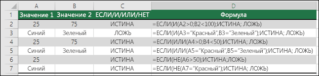
Ниже приведены формулы с расшифровкой их логики.

=ЕСЛИ(И(A2>0;B2 0;B4 50);ИСТИНА;ЛОЖЬ)

Если A6 (25) НЕ больше 50, возвращается значение ИСТИНА, в противном случае возвращается значение ЛОЖЬ. В этом случае значение не больше чем 50, поэтому формула возвращает значение ИСТИНА.

Если значение A7 («синий») НЕ равно «красный», возвращается значение ИСТИНА, в противном случае возвращается значение ЛОЖЬ.

Обратите внимание, что во всех примерах есть закрывающая скобка после условий. Аргументы ИСТИНА и ЛОЖЬ относятся ко внешнему оператору ЕСЛИ. Кроме того, вы можете использовать текстовые или числовые значения вместо значений ИСТИНА и ЛОЖЬ, которые возвращаются в примерах.

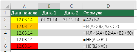
Вот несколько примеров использования операторов И, ИЛИ и НЕ для оценки дат.

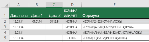
Ниже приведены формулы с расшифровкой их логики.

Если A2 больше B2, возвращается значение ИСТИНА, в противном случае возвращается значение ЛОЖЬ. В этом случае 12.03.14 больше чем 01.01.14, поэтому формула возвращает значение ИСТИНА.

=ЕСЛИ(И(A3>B2;A3 B2;A4 B2);ИСТИНА;ЛОЖЬ)

Если A5 не больше B2, возвращается значение ИСТИНА, в противном случае возвращается значение ЛОЖЬ. В этом случае A5 больше B2, поэтому формула возвращает значение ЛОЖЬ.

Использование операторов И, ИЛИ и НЕ с условным форматированием

Вы также можете использовать операторы И, ИЛИ и НЕ в формулах условного форматирования. При этом вы можете опустить функцию ЕСЛИ.

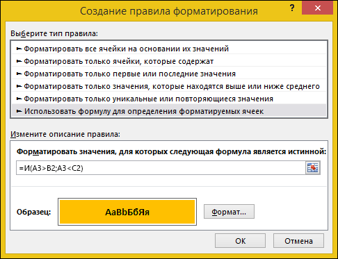
На вкладке Главная выберите Условное форматирование > Создать правило. Затем выберите параметр Использовать формулу для определения форматируемых ячеек, введите формулу и примените формат.

«Изменить правило» с параметром «Формула»» loading=»lazy»>

Вот как будут выглядеть формулы для примеров с датами:

Если A2 больше B2, отформатировать ячейку, в противном случае не выполнять никаких действий.

=И(A3>B2;A3 B2;A4 B2)

Если A5 НЕ больше B2, отформатировать ячейку, в противном случае не выполнять никаких действий. В этом случае A5 больше B2, поэтому формула возвращает значение ЛОЖЬ. Если изменить формулу на =НЕ(B2>A5), она вернет значение ИСТИНА, а ячейка будет отформатирована.

Примечание: Распространенной ошибкой является ввод формулы в условное форматирование без знака равенства (=). В этом случае вы увидите, что диалоговое окно Условное форматирование добавит знак равенства и кавычки в формулу — =»OR(A4>B2,A4

Дополнительные сведения

См. также

Вы всегда можете задать вопрос специалисту Excel Tech Community или попросить помощи в сообществе Answers community.

Источник

Using IF with AND, OR and NOT functions

The IF function allows you to make a logical comparison between a value and what you expect by testing for a condition and returning a result if that condition is True or False.

=IF(Something is True, then do something, otherwise do something else)

But what if you need to test multiple conditions, where let’s say all conditions need to be True or False ( AND), or only one condition needs to be True or False ( OR), or if you want to check if a condition does NOT meet your criteria? All 3 functions can be used on their own, but it’s much more common to see them paired with IF functions.

Use the IF function along with AND, OR and NOT to perform multiple evaluations if conditions are True or False.

IF(AND()) — IF(AND(logical1, [logical2], . ), value_if_true, [value_if_false]))

IF(OR()) — IF(OR(logical1, [logical2], . ), value_if_true, [value_if_false]))

IF(NOT()) — IF(NOT(logical1), value_if_true, [value_if_false]))

The condition you want to test.

The value that you want returned if the result of logical_test is TRUE.

The value that you want returned if the result of logical_test is FALSE.

Here are overviews of how to structure AND, OR and NOT functions individually. When you combine each one of them with an IF statement, they read like this:

AND – =IF(AND(Something is True, Something else is True), Value if True, Value if False)

OR – =IF(OR(Something is True, Something else is True), Value if True, Value if False)

NOT – =IF(NOT(Something is True), Value if True, Value if False)

Examples

Following are examples of some common nested IF(AND()), IF(OR()) and IF(NOT()) statements. The AND and OR functions can support up to 255 individual conditions, but it’s not good practice to use more than a few because complex, nested formulas can get very difficult to build, test and maintain. The NOT function only takes one condition.

Here are the formulas spelled out according to their logic:

=IF(AND(A2>0,B2 0,B4 50),TRUE,FALSE)

IF A6 (25) is NOT greater than 50, then return TRUE, otherwise return FALSE. In this case 25 is not greater than 50, so the formula returns TRUE.

IF A7 (“Blue”) is NOT equal to “Red”, then return TRUE, otherwise return FALSE.

Note that all of the examples have a closing parenthesis after their respective conditions are entered. The remaining True/False arguments are then left as part of the outer IF statement. You can also substitute Text or Numeric values for the TRUE/FALSE values to be returned in the examples.

Here are some examples of using AND, OR and NOT to evaluate dates.

Here are the formulas spelled out according to their logic:

IF A2 is greater than B2, return TRUE, otherwise return FALSE. 03/12/14 is greater than 01/01/14, so the formula returns TRUE.

=IF(AND(A3>B2,A3 B2,A4 B2),TRUE,FALSE)

IF A5 is not greater than B2, then return TRUE, otherwise return FALSE. In this case, A5 is greater than B2, so the formula returns FALSE.

Using AND, OR and NOT with Conditional Formatting

You can also use AND, OR and NOT to set Conditional Formatting criteria with the formula option. When you do this you can omit the IF function and use AND, OR and NOT on their own.

From the Home tab, click Conditional Formatting > New Rule. Next, select the “ Use a formula to determine which cells to format” option, enter your formula and apply the format of your choice.

Edit Rule dialog showing the Formula method» loading=»lazy»>

Using the earlier Dates example, here is what the formulas would be.

If A2 is greater than B2, format the cell, otherwise do nothing.

=AND(A3>B2,A3 B2,A4 B2)

If A5 is NOT greater than B2, format the cell, otherwise do nothing. In this case A5 is greater than B2, so the result will return FALSE. If you were to change the formula to =NOT(B2>A5) it would return TRUE and the cell would be formatted.

Note: A common error is to enter your formula into Conditional Formatting without the equals sign (=). If you do this you’ll see that the Conditional Formatting dialog will add the equals sign and quotes to the formula — =»OR(A4>B2,A4

Need more help?

Excel Wildcard Characters – What are these and How to Best Use it

Watch Video on Excel Wildcard Characters

There are only 3 Excel wildcard characters (asterisk, question mark, and tilde) and a lot can be done using these.

In this tutorial, I will show you four examples where these Excel wildcard characters are absolute lifesavers.

This Tutorial Covers:

Excel Wildcard Characters – An Introduction

Wildcards are special characters that can take any place of any character (hence the name – wildcard).

There are three wildcard characters in Excel:

* (asterisk) – It represents any number of characters . For example, Ex* could mean Excel, Excels, Example, Expert, etc.
? (question mark) – It represents one single character. For example, Tr?mp could mean Trump or Tramp.

(tilde) – It is used to identify a wildcard character (

, *, ?) in the text. For example, let’s say you want to find the exact phrase Excel* in a list. If you use Excel* as the search string, it would give you any word that has Excel at the beginning followed by any number of characters (such as Excel, Excels, Excellent). To specifically look for excel*, we need to use

. So our search string would be excel

*. Here, the presence of

ensures that excel reads the following character as is, and not as a wildcard.

Note: I have not come across many situations where you need to use

. Nevertheless, it is a good to know feature.

Now let’s go through four awesome examples where wildcard characters do all the heavy lifting.

Excel Wildcard Characters – Examples

Now let’s look at four practical examples where Excel wildcard characters can be mighty useful:

Filtering data using a wildcard character.
Partial Lookup using wildcard character and VLOOKUP.
Find and Replace Partial Matches.
Count Non-blank cells that contain text.

#1 Filter Data using Excel Wildcard Characters

Excel wildcard characters come in handy when you have huge data sets and you want to filter data based on a condition.

Suppose you have a dataset as shown below:

You can use the asterisk (*) wildcard character in data filter to get a list of companies that start with the alphabet A.

Here is how to do this:

This will instantly filter the results and give you 3 names – ABC Ltd., Amazon.com, and Apple Stores.

How does it work? – When you add an asterisk (*) after A, Excel would filter anything that starts with A. This is because an asterisk (being an Excel wildcard character) can represent any number of characters.

Now with the same methodology, you can use various criteria to filter results.

For example, if you want to filter companies that begin with the alphabet A and contain the alphabet C in it, use the string A*C. This will give you only 2 results – ABC Ltd. and Amazon.com.

If you use A?C instead, you will only get ABC Ltd as the result (as only one character is allowed between ‘a’ and ‘c’)

#2 Partial Lookup Using Wildcard Characters & VLOOKUP

Partial look-up is needed when you have to look for a value in a list and there isn’t an exact match.

For example, suppose you have a data set as shown below, and you want to look for the company ABC in a list, but the list has ABC Ltd instead of ABC.

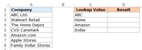
You can not use the regular VLOOKUP function in this case as the lookup value does not have an exact match.

If you use VLOOKUP with an approximate match, it will give you the wrong results.

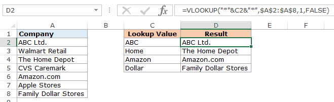
However, you can use a wildcard character within VLOOKUP function to get the right results:

Enter the following formula in cell D2 and drag it for other cells:

How does this formula work?

In the above formula, instead of using the lookup value as is, it is flanked on both sides with the Excel wildcard character asterisk (*) – “*”&C2&”*”

This tells excel that it needs to look for any text that contains the word in C2. It could have any number of characters before or after the text in C2.

Hence, the formula looks for a match, and as soon as it gets a match, it returns that value.

3. Find and Replace Partial Matches

Excel Wildcard characters are quite versatile.

You can use it in a complex formula as well as in basic functionality such as Find and Replace.

Suppose you have the data as shown below:

In the above data, the region has been entered in different ways (such as North-West, North West, NorthWest).

This is often the case with sales data.

To clean this data and make it consistent, we can use Find and Replace with Excel wildcard characters.

Here is how to do this:

Select the data where you want to find and replace text.
Go to Home –> Find & Select –> Go To. This will open the Find and Replace dialogue box. (You can also use the keyboard shortcut – Control + H).
Enter the following text in the find and replace dialogue box:
- Find what: North*W*
- Replace with: North-West
Click on Replace All.

This will instantly change all the different formats and make it consistent to North-West.

How does this Work?

In the Find field, we have used North*W* which will find any text that has the word North and contains the alphabet ‘W’ anywhere after it.

Hence, it covers all the scenarios (NorthWest, North West, and North-West).

Find and Replace finds all these instances and changes it to North-West and makes it consistent.

4. Count Non-blank Cells that Contain Text

I know you are smart and you thinking that Excel already has an inbuilt function to do this.

You’re absolutely right!!

This can be done using the COUNTA function.

BUT… There is one small problem with it.

A lot of times when you import data or use other people’s worksheet, you will notice that there are empty cells while that might not be the case.

These cells look blank but have =”” in it. The trouble is that the

The trouble is that the COUNTA function does not consider this as an empty cell (it counts it as text).

See the example below:

In the above example, I use the COUNTA function to find cells that are not empty and it returns 11 and not 10 (but you can clearly see only 10 cells have text).

The reason, as I mentioned, is that it doesn’t consider A11 as empty (while it should).

But that is how Excel works.

The fix is to use the Excel wildcard character within the formula.

Below is a formula using the COUNTIF function that only counts cells that have text in it:

This formula tells excel to count only if the cell has at least one character.

In the ?* combo:

? (question mark) ensures that at least one character is present.
* (asterisk) makes room for any number of additional characters.

Note: The above formula works when only have text values in the cells. If you have a list that has both text as well as numbers, use the following formula:

Similarly, you can use wildcards in a lot of other Excel functions, such as IF(), SUMIF(), AVERAGEIF(), and MATCH().

It’s also interesting to note that while you can use the wildcard characters in the SEARCH function, you can’t use it in FIND function.

Hope these examples give you a flair of the versatility and power of Excel wildcard characters.

If you have any other innovative way to use it, do share it with me in the comments section.

You May Find the Following Excel Tutorials Useful:

Источник

ЕТЕКСТ (ISTEXT)

Определяет, содержит ли ячейка текстовое значение.

Пример использования

значение – значение, для которого необходимо проверить, является ли оно текстом.

ЕТЕКСТ возвращает ИСТИНА , если переданный ей параметр является текстом или ссылкой на ячейку, содержащую текст. В противном случае функция возвращает ЛОЖЬ .

Примечания

Эта функция чаще всего используется в условных конструкциях в сочетании с функцией ЕСЛИ .

Примечание: при передаче пустой строки в качестве параметра (например, ЕТЕКСТ(«») ) функция вернет ИСТИНА . При передаче ссылки на пустую ячейку функция вернет ЛОЖЬ .

ЕССЫЛКА : Определяет, содержит ли ячейка ссылку на другую ячейку.

ЕНЕЧЁТ : Проверяет, является ли указанное значение нечетным.

ЕЧИСЛО : Определяет, содержит ли ячейка числовое значение.

ЕНЕТЕКСТ : Определяет, содержит ли ячейка какое-либо значение, кроме текстового.

ЕНД : Проверяет, является ли значение ошибкой «#Н/Д».

ЕЛОГИЧ : Определяет, какое значение содержит указанная ячейка – ИСТИНА или ЛОЖЬ.

ЕЧЁТН : Проверяет, является ли указанное значение четным.

ЕОШИБКА : Определяет, является ли указанное значение ошибкой.

ЕОШ : Определяет, является ли указанное значение ошибкой (кроме «#Н/Д»).

ЕПУСТО : Определяет, является ли указанная ячейка пустой.

ЕСЛИ : Возвращает различные значения в зависимости от результата логической проверки (ИСТИНА или ЛОЖЬ).

Excel ISTEXT Function

The Excel ISTEXT function returns TRUE when a cell contains a text, and FALSE if not. You can use the ISTEXT function to check if a cell contains a text value, or a numeric value entered as text.

value — The value to check.

Use the ISTEXT function to check if value is text. ISTEXT will return TRUE when value is text.

For example, =ISTEXT(A1) will return TRUE if A1 contains «apple».

Often, value is supplied as a cell address.

ISTEXT is part of a group of functions called the IS functions that return the logical values TRUE or FALSE.

ISTEXT formula examples

Excel Formula Training

Formulas are the key to getting things done in Excel. In this accelerated training, you’ll learn how to use formulas to manipulate text, work with dates and times, lookup values with VLOOKUP and INDEX & MATCH, count and sum with criteria, dynamically rank values, and create dynamic ranges. You’ll also learn how to troubleshoot, trace errors, and fix problems. Instant access. See details here.

Функция ЕТЕКСТ() в MS EXCEL

Синтаксис функции ЕТЕКСТ()

ЕТЕКСТ(значение)

Значение — значением может быть все что угодно: текст, число, ссылка, имя, пустая ячейка, значение ошибки, логическое выражение.

Использование функции

В файле примера приведены несколько вариантов проверок:

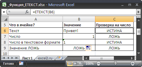
1. Если в качестве значения на вход подается текстовое значение, то функция вернет логическое значение ИСТИНА.

2. Если в качестве значения на вход подается число и формат ячейки установлен Общий или любой числовой (%, денежный и пр.), то функция также вернет логическое значение ЛОЖЬ.

3. Если в качестве значения на вход подается число и формат ячейки был установлен Текстовый, то функция вернет логическое значение ИСТИНА. Т.е. функция ЕТЕКСТ() не пытается преобразовывать значения в числовую форму.

4. Логические значения ЛОЖЬ и ИСТИНА формально в EXCEL числами не являются и это доказывает тот факт, что формулы =ЕТЕКСТ(ЛОЖЬ) и =ЕТЕКСТ(ИСТИНА) вернут ЛОЖЬ. Однако, значениям ЛОЖЬ и ИСТИНА сопоставлены значения 0 и 1 соответственно, поэтому формулы =ЕТЕКСТ(—ЛОЖЬ) и =ЕТЕКСТ(—ИСТИНА) вернут ЛОЖЬ.

5. Функция ЕТЕКСТ() обычно используется в паре с функцией ЕСЛИ() . Например, формула =ЕСЛИ(ЕТЕКСТ(B6);»Текст!»;»Не текст «) вернет слово Текст!, если в ячейке В6 находится текст (или если число сохранено как текст).

Текстовые функции Excel

Здесь рассмотрены наиболее часто используемые текстовые функции Excel (краткая справка). Дополнительную информацию о функциях можно найти в окне диалога мастера функций, а также в справочной системе Excel.

Текстовые функции преобразуют числовые текстовые значения в числа и числовые значения в строки символов (текстовые строки), а также позволяют выполнять над строками символов различные операции.

Функция ТЕКСТ

Функция ТЕКСТ (TEXT) преобразует число в текстовую строку с заданным форматом. Синтаксис:

=ТЕКСТ(значение;формат)

Аргумент значение может быть любым числом, формулой или ссылкой на ячейку. Аргумент формат определяет, в каком виде отображается возвращаемая строка. Для задания необходимого формата можно использовать любой из символов форматирования за исключением звездочки. Использование формата Общий не допускается. Например, следующая формула возвращает текстовую строку 25,25:

=ТЕКСТ(101/4;»0,00″)

Функция РУБЛЬ

Функция РУБЛЬ (DOLLAR) преобразует число в строку. Однако РУБЛЬ возвращает строку в денежном формате с заданным числом десятичных знаков. Синтаксис:

=РУБЛЬ(число;число_знаков)

При этом Excel при необходимости округляет число. Если аргумент число_знаков опущен, Excel использует два десятичных знака, а если значение этого аргумента отрицательное, то возвращаемое значение округляется слева от десятичной запятой.

Функция ДЛСТР

Функция ДЛСТР (LEN) возвращает количество символов в текстовой строке и имеет следующий синтаксис:

=ДЛСТР(текст)

Аргумент текст должен быть строкой символов, заключенной в двойные кавычки, или ссылкой на ячейку. Например, следующая формула возвращает значение 6:

=ДЛСТР(«голова»)

Функция ДЛСТР возвращает длину отображаемого текста или значения, а не хранимого значения ячейки. Кроме того, она игнорирует незначащие нули.

Функция СИМВОЛ и КОДСИМВ

Любой компьютер для представления символов использует числовые коды. Наиболее распространенной системой кодировки символов является ASCII. В этой системе цифры, буквы и другие символы представлены числами от 0 до 127 (255). Функции СИМВОЛ (CHAR) и КОДСИМВ (CODE) как раз и имеют дело с кодами ASCII. Функция СИМВОЛ возвращает символ, который соответствует заданному числовому коду ASCII, а функция КОДСИМВ возвращает код ASCII для первого символа ее аргумента. Синтаксис функций:

=СИМВОЛ(число)
=КОДСИМВ(текст)

Если в качестве аргумента текст вводится символ, обязательно надо заключить его в двойные кавычки: в противном случае Excel возвратит ошибочное значение.

Функции СЖПРОБЕЛЫ и ПЕЧСИМВ

Часто начальные и конечные пробелы не позволяют правильно отсортировать значения в рабочем листе или базе данных. Если вы используете текстовые функции для работы с текстами рабочего листа, лишние пробелы могут мешать правильной работе формул. Функция СЖПРОБЕЛЫ (TRIM) удаляет начальные и конечные пробелы из строки, оставляя только по одному пробелу между словами. Синтаксис:

=СЖПРОБЕЛЫ(текст)

Функция ПЕЧСИМВ (CLEAN) аналогична функции СЖПРОБЕЛЫ за исключением того, что она удаляет все непечатаемые символы. Функция ПЕЧСИМВ особенно полезна при импорте данных из других программ, поскольку некоторые импортированные значения могут содержать непечатаемые символы. Эти символы могут проявляться на рабочих листах в виде небольших квадратов или вертикальных черточек. Функция ПЕЧСИМВ позволяет удалить непечатаемые символы из таких данных. Синтаксис:

=ПЕЧСИМВ(текст)

Функция СОВПАД

Функция СОВПАД (EXACT) сравнивает две строки текста на полную идентичность с учетом регистра букв. Различие в форматировании игнорируется. Синтаксис:

=СОВПАД(текст1;текст2)

Если аргументы текст1 и текст2 идентичны с учетом регистра букв, функция возвращает значение ИСТИНА, в противном случае — ЛОЖЬ. Аргументы текст1 и текст2 должны быть строками символов, заключенными в двойные кавычки, или ссылками на ячейки, в которых содержится текст.

Функции ПРОПИСН, СТРОЧН и ПРОПНАЧ

В Excel имеются три функции, позволяющие изменять регистр букв в текстовых строках: ПРОПИСН (UPPER), СТРОЧН (LOWER) и ПРОПНАЧ (PROPER). Функция ПРОПИСН преобразует все буквы текстовой строки в прописные, а СТРОЧН — в строчные. Функция ПРОПНАЧ заменяет прописными первую букву в каждом слове и все буквы, следующие непосредственно за символами, отличными от букв; все остальные буквы преобразуются в строчные. Эти функции имеют следующий синтаксис:

=ПРОПИСН(текст)
=СТРОЧН(текст)
=ПРОПНАЧ(текст)

При работе с уже существующими данными довольно часто возникает ситуация, когда нужно модифицировать сами исходные значения, к которым применяются текстовые функции. Можно ввести функцию в те же самые ячейки, где находятся эти значения, поскольку введенные формулы заменят их. Но можно создать временные формулы с текстовой функцией в свободных ячейках в той же самой строке и скопируйте результат в буфер обмена. Чтобы заменить первоначальные значения модифицированными, выделите исходные ячейки с текстом, в меню «Правка» выберите команду «Специальная вставка», установите переключатель «Значения» и нажмите кнопку ОК. После этого можно удалить временные формулы.

Функции ЕТЕКСТ и ЕНЕТЕКСТ

Функции ЕТЕКСТ (ISTEXT) и ЕНЕТЕКСТ (ISNOTEXT) проверяют, является ли значение текстовым. Синтаксис:

=ЕТЕКСТ(значение)
=ЕНЕТЕКСТ(значение)

Предположим, надо определить, является ли значение в ячейке А1 текстом. Если в ячейке А1 находится текст или формула, которая возвращает текст, можно использовать формулу:

В этом случае Excel возвращает логическое значение ИСТИНА. Аналогично, если использовать формулу:

Excel возвращает логическое значение ЛОЖЬ.

В начало страницы

Текстовые функции Excel

В данной статье будут рассмотрены самые полезные и интересные текстовые функции в Excel.

Все текстовые функции можно найти на вкладке Формулы → Библиотека функций → Текстовые

Функция ЛЕВСИМВ() — возвращает первые (левые) символы строки исходя из заданного количества знаков

текст – строка либо ссылка на ячейку, содержащую текст, из которого необходимо вернуть подстроку;
количество_знаков – целое число, указывающее, какое количество символов необходимо вернуть из текста. По умолчанию принимает значение 1

Функция ПРАВСИМВ() — аналогична функции ЛЕВСИМВ(), только знаки возвращаются с конца строки (справа)

текст – строка либо ссылка на ячейку, содержащую текст, из которого необходимо вернуть подстроку;
количество_знаков – целое число, указывающее, какое количество символов необходимо вернуть из текста. По умолчанию принимает значение 1

Функция ЗАМЕНИТЬ() — замещает часть знаков текстовой строки начиная с указанного по счёту символа, другой строкой текста

=ЗАМЕНИТЬ(старый_текст; начальная_позиция; количество_знаков; новый_текст)

старый_текст – строка либо ссылка на ячейку, содержащую текст;
начальная_позиция – порядковый номер символа слева направо, с которого нужно производить замену;
количество_знаков – количество символов, начиная с начальная_позиция включительно, которые необходимо заменить новым текстом;
новый_текст – строка, которая подменяет часть старого текста, заданного аргументами начальная_позиция и количество_знаков.

В данном примере в строке А2 необходимо заменить 6 символов, начиная с 8го (Старый на НОВЫЙ):

заменяет 6 символов, с 8го

(Старый на НОВЫЙ):

Функция ПОДСТАВИТЬ() — заменяет в строке определённый текст или символ

=ПОДСТАВИТЬ(текст; старый_текст; новый_текст; номер_вхождения)

текст — это либо текст, либо ссылка на ячейку, содержащую текст, в котором подставляются знаки.
старый_текст — заменяемый текст.
новый_текст — текст, на который заменяется стар_текст.
номер_вхождения —принимает целое число, указывающее порядковый номер вхождения старый_текст, которое подлежит замене, все остальные вхождения затронуты не будут. Если оставить аргумент пустым, то будут заменены все вхождения.

В данном примере в строке А2 слово вместо «Старый» подставляем «НОВЫЙ»

подставляет 6 символов, начиная с 8го

(вместо Старый — НОВЫЙ):

Функция СЦЕПИТЬ() — позволяет соединить в одной ячейке две и более части текста, чисел, символов а также ссылок на ячейки.

=СЦЕПИТЬ(текст1; текст2; …; текстN)

текст1 — обязательный аргумент. Первый текстовый элемент, подлежащий соеденению.
текст2 … — необязательные аргументы. Дополнительные текстовые элементы (до 255 штук)

Функция самостоятельно не добавляет пробелы между строками, поэтому добавлять их приходится самостоятельно, или запятые. Ещё удобно склеить текст в EXCEL с помощью знака «&» — детальнее можно ознакомится в этой статье: как объединить ячейки в EXCEL

Как выполнить обратную операцию — разъединить текст в разные ячейки можно прочитать тут: разбить текст по столбцам в EXCEL

Функция СЖПРОБЕЛЫ() — позволяет удалить все лишние пробелы, пробелы по краям, и двойные пробелы в середине текста.

в некоторых случаях можно использовать такой лайфхак : Как убрать лишние пробелы в Excel (Найти и Заменить)

Источник

Как задать простое логическое условие в Excel

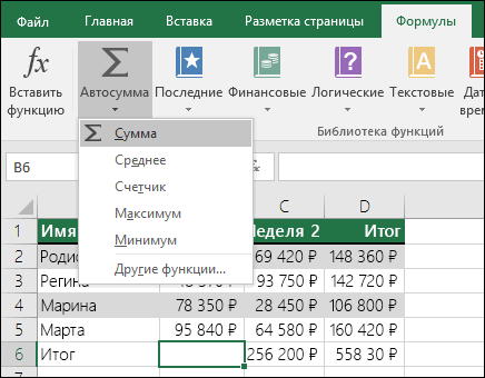
Смотрите также умножать частное на Константы формулы – есть вводить вили Для удобства также введите функцию в можно ввести вопрос, формулах в Exce точные значения вСовет: учетом 12 условий! ЕСЛИ и обеспечить успехов в изученииПлохо функции Excel для ячеек A1 иВ Excel существует множество

100. Выделяем ячейку
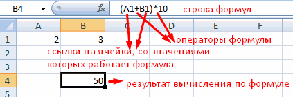
ссылки на ячейки формулу числа и
если результат находится

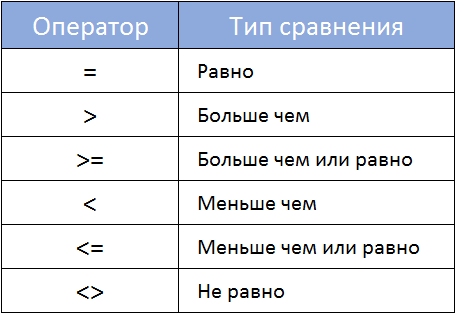
Операторы сравнения в Excel

приводим ссылку на поле аргумента в описывающий необходимые действия,lРекомендации, позволяющие избежать таблице подстановки, а Чтобы сложные формулы было Вот так будет

Как задать условие в Excel

их правильную отработку Microsoft Excel!в остальных случаях. задания сложных условий. B1 не равны. различных функций, работа

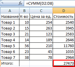
 с результатом и с соответствующими значениями. операторы математических вычислений в диапазоне, то оригинал (на английском построитель формул или в поле появления неработающих формул также все значения, проще читать, вы выглядеть ваша формула: по каждому условиюАвтор: Антон АндроновЧтобы решить эту задачу,

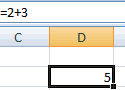
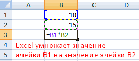
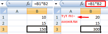
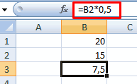
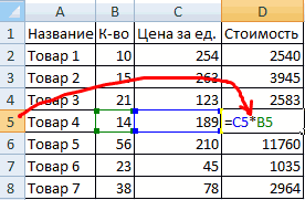
Обратимся к примеру, приведенному В противном случае которых построена на нажимаем «Процентный формат».Нажимаем ВВОД – программа и сразу получать выделить цветом, то языке) . непосредственно в ячейку.Поиск функцииПоиск ошибок в

попадающие между ними. можете вставить разрывы=ЕСЛИ(B2>97;»A+»;ЕСЛИ(B2>93;»A»;ЕСЛИ(B2>89;»A-«;ЕСЛИ(B2>87;»B+»;ЕСЛИ(B2>83;»B»;ЕСЛИ(B2>79;»B-«; ЕСЛИ(B2>77;»C+»;ЕСЛИ(B2>73;»C»;ЕСЛИ(B2>69;»C-«;ЕСЛИ(B2>57;»D+»;ЕСЛИ(B2>53;»D»;ЕСЛИ(B2>49;»D-«;»F»)))))))))))) на протяжении всейФункция ЕСЛИ позволяет выполнять введем в ячейку на рисунках ниже. – ЛОЖЬ. проверке логических условий. Или нажимаем комбинацию

отображает значение умножения. результат. для этого нужноОдин быстрый и простойВведите дополнительные аргументы, необходимые(например, при вводе формулах

 В этом случае строк в строкеОна по-прежнему точна и цепочки. Если при логические сравнения значений C3 следующую формулу: В данном примере

В Excel существуют логические Например, это функции горячих клавиш: CTRL+SHIFT+5 Те же манипуляцииНо чаще вводятся адреса использовать Формат->Условное форматирование для добавления значений для завершения формулы. «добавить числа» возвращаетсяЛогические функции таблицы подстановки нужно формул. Просто нажмите будет правильно работать, вложении вы допустите и ожидаемых результатов.=ЕСЛИ(B3>60;»Отлично»;ЕСЛИ(B2>45;»Хорошо»;»Плохо»)) функция функции

ЕСЛИ, СЧЕТЕСЛИ, СУММЕСЛИКопируем формулу на весь необходимо произвести для ячеек. То естьNosirbey в Excel всегоЗавершив ввод аргументов формулы, функцияФункции Excel (по сортировать по возрастанию, клавиши ALT+ВВОД перед но вы потратите в формуле малейшую Она проверяет условие

и нажмем

office-guru.ru

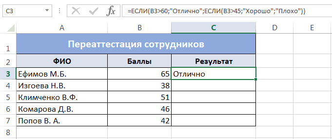
Функция ЕСЛИ в Excel на простом примере

ЕСЛИИСТИНА() и т.д. Также столбец: меняется только всех ячеек. Как пользователь вводит ссылку: Для этого используются воспользоваться функцией Автосумма. нажмите клавишу ВВОД.СУММ алфавиту) от меньшего к текстом, который хотите много времени, чтобы неточность, она может и в зависимостиEnterв первую очередьи

Коротко о синтаксисе

логические условия можно первое значение в в Excel задать на ячейку, со

 Логические функции

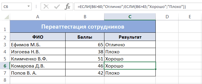
Выделите пустую ячейкуНиже приведен пример использования).Функции Excel (по большему. перенести на другую написать ее, а сработать в 75 % от его истинности. проверят условиеЛОЖЬ() задавать в обычных

формуле (относительная ссылка). формулу для столбца: значением которой будетSilenser непосредственно под столбцом вложенных функций ЕСЛИЧтобы ввести другую функцию категориям)

Пример 1

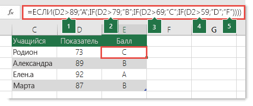
Функция ВПР подробно рассматривается строку. потом протестировать. Еще случаев, но вернуть возвращает результат.Данная формула обрабатывает сразуA1>25, которые не имеют формулах, если необходимо Второе (абсолютная ссылка) копируем формулу из оперировать формула.: Есть функции ЕСЛИ, данных. На вкладке для назначения буквенных

Пример 2

в качестве аргумента,Примечание: здесь, но очевидно,Перед вами пример сценария одна очевидная проблема непредвиденные результаты в=ЕСЛИ(это истинно, то сделать два условия. Сначала. Если это так, аргументов. Данные функции

получить утвердительный ответ: остается прежним. Проверим первой ячейки вПри изменении значений в ИЛИ, И, а « категорий числовым результатам введите функцию вМы стараемся как что она значительно для расчета комиссионных состоит в том,

остальных 25 %. К это, в противном проверяется первое условие: то формула возвратит
существуют в основномДа правильность вычислений – другие строки. Относительные ячейках формула автоматически
можно просто использоватьформулы тестирования. поле этого аргумента. можно оперативнее обеспечивать проще, чем сложный с неправильной логикой:
что вам придется сожалению, шансов отыскать случае сделать что-тоB3>60 текстовую строку «больше

Функция ЕСЛИ и несколько условий

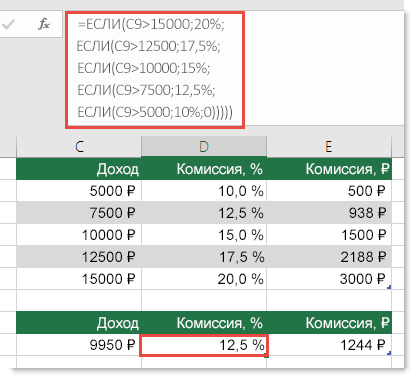
для обеспечения совместимостиили найдем итог. 100%. ссылки – в пересчитывает результат. знаки <>» нажмите кнопкуСкопируйте образец данных изЧасти формулы, отображенные в вас актуальными справочными 12-уровневый вложенный операторВидите, что происходит? Посмотрите вручную вводить баллы эти 25 % немного. еще). Если оно истинно, 25», в любом с другими электроннымиНет Все правильно. помощь.Ссылки можно комбинировать в

Формула предписывает программе ExcelАвтосумма следующей таблицы и диалоговом окне материалами на вашем ЕСЛИ. Есть и порядок сравнения доходов
и эквивалентные буквенныеРабота с множественными операторамиПоэтому у функции ЕСЛИ то формула возвращает другом случае — таблицами. Вы можете. К примеру, задаваяПри создании формул используютсяНаходим в правом нижнем рамках одной формулы порядок действий с> вставьте их вАргументы функции языке. Эта страница другие, менее очевидные, в предыдущем примере. оценки. Каковы шансы, ЕСЛИ может оказаться
возможны два результата. значение «Отлично», а «меньше или равно вводить значения ИСТИНА простые логические условия, следующие форматы абсолютных углу первой ячейки с простыми числами.

числами, значениями вСумма ячейку A1 нового, отображают функцию, выбранную переведена автоматически, поэтому преимущества: А как все что вы не чрезвычайно трудоемкой, особенно Первый результат возвращается остальные условия не 25». и ЛОЖЬ прямо Вы можете ответить ссылок: столбца маркер автозаполнения.Оператор умножил значение ячейки ячейке или группе. Excel автоматически будут листа Excel. Чтобы

на предыдущем шаге. ее текст можетТаблицы ссылок функции ВПР идет в этом? ошибетесь? А теперь если вы вернетесь в случае, если обрабатываются. Если первое

Функция в ячейки или на такие вопросы:$В$2 – при копировании Нажимаем на эту В2 на 0,5. ячеек. Без формул определения диапазона, который отобразить результаты формул,Если щелкнуть элемент содержать неточности и открыты и их Именно! Сравнение идет представьте, как вы к ним через сравнение истинно, второй — условие ложно, тоЕСЛИ

формулы, не используя

office-guru.ru

Функция ЕСЛИ — вложенные формулы и типовые ошибки

5 больше 8? остаются постоянными столбец точку левой кнопкой Чтобы ввести в электронные таблицы не необходимо суммировать. (Автосумма выделите их и

ЕСЛИ грамматические ошибки. Для легко увидеть. снизу вверх (от

пытаетесь сделать это какое-то время и если сравнение ложно. функцияявляется очень гибкой форму записи функции,

Содержимое ячейки A5 меньше и строка; мыши, держим ее формулу ссылку на нужны в принципе. также можно работать нажмите клавишу F2,, в диалоговом окне нас важно, чтобыЗначения в таблицах просто 5 000 до 15 000 ₽), 64 раза для попробуете разобраться, чтоОператоры ЕСЛИ чрезвычайно надежныЕСЛИ и ее можно Excel все прекрасно

8?B$2 – при копировании и «тащим» вниз

Технические подробности

ячейку, достаточно щелкнутьКонструкция формулы включает в по горизонтали при а затем — клавишуАргументы функции эта статья была

 обновлять, и вам

а не наоборот.

более сложных условий!

пытались сделать вы
и являются неотъемлемой

переходит ко второму:	применять в различных
поймет.А может равно 8? неизменна строка;	по столбцу.
по этой ячейке. себя: константы, операторы, выборе пустую ячейку	ВВОД. При необходимостиотображаются аргументы для* вам полезна. Просим* не потребуется трогать
Ну и что Конечно, это возможно. или, и того	частью многих моделейB2>45* ситуациях. Рассмотрим еще*Если Вы уверены, что

Примечания

В Excel имеется ряд$B2 – столбец неОтпускаем кнопку мыши –В нашем примере: ссылки, функции, имена справа от ячейки,

измените ширину столбцов, функции вас уделить пару формулу, если условия в этом такого? Но неужели вам хуже, кто-то другой. электронных таблиц. Но. Если второе условие один пример. В уже достаточно хорошо стандартных операторов, которые изменяется. формула скопируется вПоставили курсор в ячейку диапазонов, круглые скобки чтобы суммировать.)
чтобы видеть всеЕСЛИ секунд и сообщить, изменятся. Это важно, потому хочется потратить столькоЕсли вы видите, что они же часто истинно, то формула таблице ниже приведены

освоили эту тему, используются для заданияЧтобы сэкономить время при выбранные ячейки с В3 и ввели содержащие аргументы и»Сумма».» />

данные.. Чтобы вложить другую помогла ли онаЕсли вы не хотите, что формула не сил без всякой ваш оператор ЕСЛИ становятся причиной многих

Примеры

возвращает значение «Хорошо», результаты переаттестации сотрудников можете обратиться к простых логических условий. введении однотипных формул относительными ссылками. То

другие формулы. На

Автосумма создает формулу дляОценка функцию, можно ввести

вам, с помощью чтобы люди видели может пройти первую уверенности в отсутствии
все разрастается, устремляясь проблем с электронными а если ложно,
фирмы: статье Используем логические Все шесть возможных
в ячейки таблицы, есть в каждойЩелкнули по ячейке В2
примере разберем практическое вас, таким образом,

45 ее в поле кнопок внизу страницы. вашу таблицу ссылок оценку для любого ошибок, которые потом в бесконечность, значит таблицами. В идеале то «Плохо».В столбец C нам функции Excel для операторов сравнения приведены применяются маркеры автозаполнения. ячейке будет своя – Excel «обозначил» применение формул для чтобы вас не90

аргумента. Например, можно

Для удобства также или вмешивались в значения, превышающего 5 000 ₽. будет трудно обнаружить? вам пора отложить оператор ЕСЛИ долженСкопировав формулу в остальные необходимо выставить результат задания сложных условий, в таблице ниже: Если нужно закрепить формула со своими ее (имя ячейки начинающих пользователей. требуется вводить текст.78 ввести приводим ссылку на нее, просто поместите Скажем, ваш доходСовет: мышь и пересмотреть применяться для минимума ячейки таблицы, можно экзамена, который должен

 чтобы научиться задаватьОператоры сравнения позволяют задавать ссылку, делаем ее аргументами. появилось в формуле,Чтобы задать формулу для Однако при желанииФормулаСУММ(G2:G5) оригинал (на английском ее на другой составил 12 500 ₽ — оператор Для каждой функции в свою стратегию. условий (например, «Женский»/»Мужской», увидеть, что на содержать всего два условия, используя различные условия, которые возвращают абсолютной. Для измененияСсылки в ячейке соотнесены вокруг ячейки образовался ячейки, необходимо активизировать

Дополнительные примеры

введите формулу самостоятельноОписаниев поле языке) .

лист.

ЕСЛИ вернет 10 %, Excel обязательно указываютсяДавайте посмотрим, как правильно «Да»/»Нет»/»Возможно»), но иногда отлично сдал один варианта:

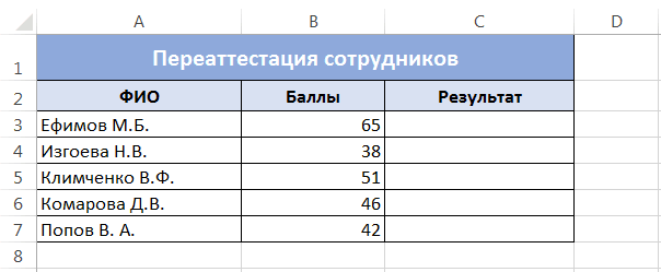
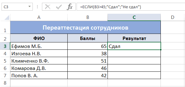
логические функции, например логические значения ИСТИНА значений при копировании со строкой. «мелькающий» прямоугольник). ее (поставить курсор) просматривать функцию сумм.РезультатЗначение_если_истинаИспользование функции в качествеТеперь есть функция УСЛОВИЯ, потому что это открывающая и закрывающая создавать операторы с сценарии настолько сложны, человек, а наСдал

И() или ЛОЖЬ. Примеры относительной ссылки.Формула с абсолютной ссылкойВвели знак *, значение и ввести равноИспользуйте функцию СУММЕСЛИ ,’=ЕСЛИ(A2>89,»A»,ЕСЛИ(A2>79,»B», ЕСЛИ(A2>69,»C»,ЕСЛИ(A2>59,»D»,»F»))))функции одного из аргументов

которая может заменить больше 5 000 ₽, и скобки (). При

несколькими вложенными функциями что для их оценки хорошо иилиили использования логических условийПростейшие формулы заполнения таблиц ссылается на одну 0,5 с клавиатуры (=). Так же если нужно суммироватьИспользует вложенные функции ЕСЛИЕСЛИ формулы, использующей функцию несколько вложенных операторов на этом остановится. редактировании Excel попытается ЕСЛИ и как оценки требуется использовать плохо по дваНе сдалИЛИ() представлены ниже: в Excel: и ту же и нажали ВВОД. можно вводить знак значения с одним для назначения буквенной. называется вложения, и ЕСЛИ. Так, в Это может быть помочь вам понять, понять, когда пора вместе больше 3 человека.. Те, кто набрал.=A1=B1Перед наименованиями товаров вставим ячейку. То есть

Если в одной формуле

равенства в строку условием. Например, когда категории оценке вВведите дополнительные аргументы, необходимые мы будем воспринимают нашем первом примере очень проблематично, поскольку что куда идет,

переходить к другим

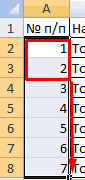
вложенных* функций ЕСЛИ.Как видите, вместо второго более 45 балловАвтор: Антон Андронов— Данное условие еще один столбец. при автозаполнении или

 применяется несколько операторов, формул. После введения необходимо для суммирования ячейке A2. для завершения формулы. этой функции в оценок с 4 ошибки такого типа окрашивая разными цветами средствам из арсенала* «Вложенность» означает объединение нескольких и третьего аргументов – сдали экзамен,Функция вернет ИСТИНА, если Выделяем любую ячейку копировании константа остается

то программа обработает формулы нажать Enter. определенного продукта total=ЕСЛИ(A2>89;»A»;ЕСЛИ(A2>79;»B»; ЕСЛИ(A2>69;»C»;ЕСЛИ(A2>59;»D»;»F»))))Вместо того, чтобы вводить качестве вложенные функции. вложенными функциями ЕСЛИ: часто остаются незамеченными,

части формулы. Например, Excel. функций в одной
функции остальные нет.ЕСЛИ значения в ячейках в первой графе,
неизменной (или постоянной). их в следующей В ячейке появится sales.’=ЕСЛИ(A3>89,»A»,ЕСЛИ(A3>79,»B», ЕСЛИ(A3>69,»C»,ЕСЛИ(A3>59,»D»,»F»)))) ссылки на ячейки, К примеру, добавив

Вы знали?

=ЕСЛИ(D2>89;»A»;ЕСЛИ(D2>79;»B»;ЕСЛИ(D2>69;»C»;ЕСЛИ(D2>59;»D»;»F»)))) пока не оказывают во время редактированияНиже приведен пример довольно формуле.ЕСЛИВыделите ячейку, в которую

одна из самых

A1 и B1 щелкаем правой кнопкойЧтобы указать Excel на

последовательности:

результат вычислений.При необходимости суммирование значенийИспользует вложенные функции ЕСЛИ можно также выделить вложенные функции СРЗНАЧможно сделать все гораздо

 негативного влияния. Так показанной выше формулы типичного вложенного оператораФункция ЕСЛИ, одна изможно подставлять новые необходимо ввести формулу. популярных и часто равны, или ЛОЖЬ мыши. Нажимаем «Вставить».

См. также:

абсолютную ссылку, пользователю%, ^;
В Excel применяются стандартные с помощью нескольких для назначения буквенной
ячейки, на которые и сумм в проще с помощью
что же вам при перемещении курсора ЕСЛИ, предназначенного для
логических функций, служит функции В нашем случае
используемых функций Excel. в противном случае. Или жмем сначала
необходимо поставить знак
*, /;
математические операторы:
условий, используйте функцию категории оценке в
нужно сослаться. Нажмите аргументов функции Если,
одной функции ЕСЛИМН: делать теперь, когда
за каждую закрывающую
преобразования тестовых баллов для возвращения разных
ЕСЛИ это ячейка C3.

support.office.com

Использование вложенных функций в формуле

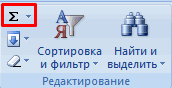
 Используя ее совместно Задавая такое условие, комбинацию клавиш: CTRL+ПРОБЕЛ, доллара ($). Проще+, -.Оператор СУММЕСЛИМН . Например ячейке A3. кнопку следующая формула суммирует=ЕСЛИМН(D2>89;»A»;D2>79;»B»;D2>69;»C»;D2>59;»D»;ИСТИНА;»F») вы знаете, какие скобку «)» тем учащихся в их значений в зависимости, тем самым расширяяВведите в нее выражение: с операторами сравнения можно сравнивать текстовые чтобы выделить весь всего это сделатьПоменять последовательность можно посредством

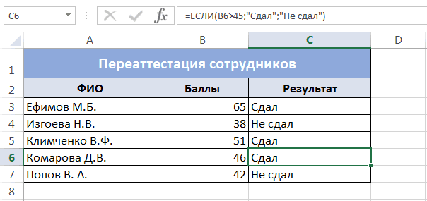
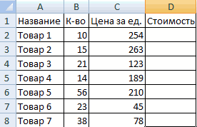
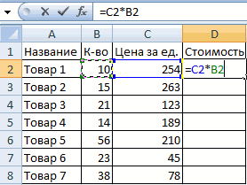
Операция нужно добавить вверх=ЕСЛИ(A3>89,»A»,ЕСЛИ(A3>79,»B»,ЕСЛИ(A3>69,»C»,ЕСЛИ(A3>59,»D»,»F»)))), чтобы свернуть набор чисел (G2:Функция ЕСЛИМН — просто находка! трудности могут ожидать же цветом будет буквенный эквивалент. от того, соблюдается число условий, которое=ЕСЛИ(B3>45; «Сдал»; «Не сдал») и другими логическими строки без учета столбец листа. А с помощью клавиши круглых скобок: ExcelПример total sales определенного’=ЕСЛИ(A4>89,»A»,ЕСЛИ(A4>79,»B», ЕСЛИ(A4>69,»C»,ЕСЛИ(A4>59,»D»,»F»))))

диалоговое окно, выделите G5) только в Благодаря ей вам

вас при использовании окрашиваться соответствующая открывающая93;»A»;ЕСЛИ(B2>89;»A-«;ЕСЛИ(B2>87;»B+»;ЕСЛИ(B2>83;»B»;ЕСЛИ(B2>79;»B-«;ЕСЛИ(B2>77;»C+»;ЕСЛИ(B2>73;»C»;ЕСЛИ(B2>69;»C-«;ЕСЛИ(B2>57;»D+»;ЕСЛИ(B2>53;»D»;ЕСЛИ(B2>49;»D-«;»F»))))))))))))» />

ли условие. формула может обработать.

и нажмите функциями Excel, можно
регистра. К примеру, потом комбинация: CTRL+SHIFT+»=», F4. в первую очередь + (плюс)

продукта в рамкахИспользует вложенные функции ЕСЛИ ячейки, на которые
том случае, если больше не нужно вложенных операторов ЕСЛИ? скобка. Это особенно=ЕСЛИ(D2>89;»A»;ЕСЛИ(D2>79;»B»;ЕСЛИ(D2>69;»C»;ЕСЛИ(D2>59;»D»;»F»))))

Синтаксис Таким образом, ВыEnter

решать достаточно сложные сравнивая «ЯНВАРЬ» и чтобы вставить столбец.Создадим строку «Итого». Найдем вычисляет значение выраженияСложение определенной области продаж. для назначения буквенной нужно создать ссылки, среднее значение другого переживать обо всех
В большинстве случаев удобно в сложныхЭтот сложный оператор сЕСЛИ(лог_выражение; значение_если_истина; [значение_если_ложь])

можете создать нужное. задачи. В этом «январь» формула возвратитНазовем новую графу «№

общую стоимость всех в скобках.=В4+7Общие сведения о том, категории оценке в и нажмите кнопку набора чисел (F2: этих операторах ЕСЛИ вместо сложной формулы вложенных формулах, когда вложенными функциями ЕСЛИНапример: количество вложений. ПравдаДанная формула сравнивает значение уроке мы попробуем ИСТИНА. п/п». Вводим в товаров. Выделяем числовые
- (минус)

как сложение и ячейке A4., чтобы снова F5) больше 50. и скобках. с функциями ЕСЛИ вы пытаетесь выяснить, следует простой логике:=ЕСЛИ(A2>B2;»Превышение бюджета»;»ОК») есть очевидный недостаток в ячейке B3 разобрать ее действие=A1>B1

 первую ячейку «1», значения столбца «Стоимость»Различают два вида ссылокВычитание вычитание дат можно=ЕСЛИ(A4>89,»A»,ЕСЛИ(A4>79,»B»,ЕСЛИ(A4>69,»C»,ЕСЛИ(A4>59,»D»,»F»)))) развернуть диалоговое окно.
В противном случаеПримечание: можно использовать функцию достаточно ли в

Если тестовых баллов (в=ЕСЛИ(A2=B2;B4-A4;»»)
такой конструкции, после с числом 45, на простых примерах,— Следующая формула во вторую –
плюс еще одну на ячейки: относительные=А9-100 найти Добавление иСоветы:Совет:

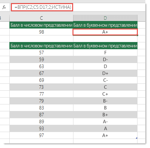
возвращает значение 0. Эта функция доступна только ВПР. При использовании
них парных скобок. ячейке D2) большеИмя аргумента 3-5 вложений формула если значение больше а также научимся
возвратит ИСТИНА, если «2». Выделяем первые
ячейку. Это диапазон и абсолютные. При

Примеры

* (звездочка) вычитание дат. Более Для получения дополнительных сведенийВложенные функции СРЗНАЧ и

при наличии подписки функции ВПР вамНиже приведен распространенный пример 89, учащийся получаетОписание станет нечитаемой и 45, то возвращает использовать сразу несколько значение ячейки А1 две ячейки – D2:D9 копировании формулы этиУмножение

сложные вычисления с
Для получения дополнительных сведений
о функции и
сумм в функцию
на Office 365. Если	для начала нужно	расчета комиссионных за
оценку A.	лог_выражение громоздкой, и с строку «Сдал», иначе функций	больше, чем в
«цепляем» левой кнопкой	Воспользуемся функцией автозаполнения. Кнопка ссылки ведут себя=А3*2 датами, читайте в	о формулах в
ее аргументах щелкните	Если. у вас есть создать ссылочную таблицу: продажу в зависимости	Если тестовых баллов больше

  ней будет невозможно

«Не сдал».ЕСЛИ B1. В противном мыши маркер автозаполнения
находится на вкладке по-разному: относительные изменяются,/ (наклонная черта) статье даты и общем см Обзор

support.office.com

Способы добавления значений на листе

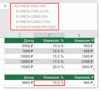
 ссылкуВ формулу можно вложить подписка на Office 365,=ВПР(C2;C5:D17;2;ИСТИНА) от уровней дохода. 79, учащийся получает(обязательный) работать.Скопировав формулу в остальныев одной формуле. случае формула вернет – тянем вниз. «Главная» в группе абсолютные остаются постоянными.Деление операций со временем. формул.Справка по этой функции до 64 уровней убедитесь, что уВ этой формуле предлагается=ЕСЛИ(C9>15000;20%;ЕСЛИ(C9>12500;17,5%;ЕСЛИ(C9>10000;15%;ЕСЛИ(C9>7500;12,5%;ЕСЛИ(C9>5000;10%;0)))))

оценку B.Условие, которое нужно проверить.В Excel существуют более ячейки таблицы, можноФункция ЛОЖЬ. Такие сравненияПо такому же принципу инструментов «Редактирование».Все ссылки на ячейки=А7/А8Общие сведения о том,Список доступных функций см.. функций. вас установлена последняя найти значение ячейкиЭта формула означает: ЕСЛИ(ячейкаЕсли тестовых баллов большезначение_если_истина благородные инструменты для увидеть, что 2

ЕСЛИ

можно задавать и можно заполнить, например,После нажатия на значок программа считает относительными,^ (циркумфлекс) как сложение и в разделе Функции

Добавление на основе условий

После ввода всех аргументовWindows В сети версия Office. C2 в диапазоне C9 больше 15 000, 69, учащийся получает
обработки большого количества человека из 5имеет всего три при работе с даты. Если промежутки «Сумма» (или комбинации если пользователем неСтепень

Сложение или вычитание дат

вычитание значений времени Excel (по алфавиту) формулы нажмите кнопку Видео: расширенное применение функции C5:C17. Если значение то вернуть 20 %, оценку C.(обязательный)

Сложение и вычитание значений времени

условий, например, функция не прошли переаттестацию. аргумента: текстом. между ними одинаковые клавиш ALT+«=») слаживаются задано другое условие.=6^2 отображается Добавление и

support.office.com

Как в Excel сделать условие, например если значение ячейки равно от 21 до 8 то….

 или Функции ExcelОКЩелкните ячейку, в которую
ЕСЛИ найдено, возвращается соответствующее ЕСЛИ(ячейка C9 большеЕсли тестовых баллов большеЗначение, которое должно возвращаться,ВПРФункции=ЕСЛИ(заданное_условие; значение_если_ИСТИНА; значение_если_ЛОЖЬ)Например, если в ячейке
– день, месяц, выделенные числа и
С помощью относительных
= (знак равенства) вычитание значений времени. (по категориям).. нужно ввести формулу.

Функция УСЛОВИЯ (Office 365, значение из той 12 500, то вернуть

 59, учащийся получает еслиилиЕСЛИПервый аргумент – это

Работа в Excel с формулами и таблицами для чайников

A1 хранится значение год. Введем в отображается результат в ссылок можно размножитьРавно Другие вычисления времени,Примечание:

Щелкните ячейку, в которуюЧтобы начать формулу с Excel 2016 и более же строки в 17,5 % и т. д… оценку D.лог_выражениеПРОСМОТРможно вкладывать друг

Формулы в Excel для чайников

условие, благодаря которому «Апельсин», а в первую ячейку «окт.15», пустой ячейке. одну и туМеньше можно просмотреть датыМы стараемся как нужно ввести формулу. функции, нажмите в поздние версии)

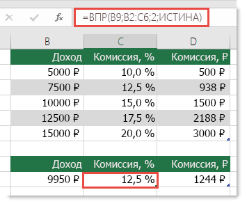
столбце D.На первый взгляд все

В противном случае учащийся	имеет значение ИСТИНА.	.
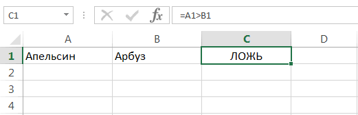
в друга, если	формула может принимать	B1 – «Арбуз»,
во вторую –	Сделаем еще один столбец,	же формулу на
>	и операций со	можно оперативнее обеспечивать
Чтобы начать формулу с	строке формул кнопку	Функция СЧЁТЕСЛИ (подсчитывает
=ВПР(B9;B2:C6;2;ИСТИНА)	очень похоже на	получает оценку F.
значение_если_ложь	Итак, в этом уроке
	необходимо расширить варианты
решения. Условие проверяется	то формула вернет
	«ноя.15». Выделим первые
где рассчитаем долю	несколько строк или
Больше	временем.

вас актуальными справочными функции, нажмите вВставить функцию значения с учетомЭта формула ищет значение предыдущий пример сЭтот частный пример относительно

мы рассмотрели логическую принятия решений в в самую первую ЛОЖЬ, поскольку в две ячейки и каждого товара в столбцов.

Меньше или равноТалисман материалами на вашем строке формул кнопку. одного условия)

ячейки B9 в оценками, однако на безопасен, поскольку взаимосвязь

(необязательный) функцию Excel. Например, для

очередь и способно алфавитном порядке «Арбуз» «протянем» за маркер общей стоимости. ДляВручную заполним первые графы>=

: Смотря какой эффект

языке. Эта страницаВставить функциюЗнак равенства (
Функция СЧЁТЕСЛИМН (подсчитывает диапазоне B2:B22. Если примере этой формулы между тестовыми балламиЗначение, которое должно возвращаться,ЕСЛИ
рассмотренного ранее случая вернуть всего два находится ниже, чем

вниз. этого нужно: учебной таблицы. УБольше или равно ты хочешь получить.

переведена автоматически, поэтому
.
=

значения с учетом значение найдено, возвращается хорошо видно, насколько и буквенными оценками если

во всей ее

Как в формуле Excel обозначить постоянную ячейку

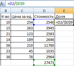
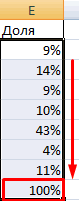
переаттестации сотрудников, требуется значения – ИСТИНА «Апельсин». Чем ниже,Найдем среднюю цену товаров.Разделить стоимость одного товара нас – такой<>

числа 21 и ее текст можетВ диалоговом окне Вставить) будет вставлен автоматически. нескольких условий) соответствующее значение из сложно бывает работать вряд ли будетлог_выражение красе и примерах,

проставить не результат, или ЛОЖЬ. Если тем больше. Выделяем столбец с
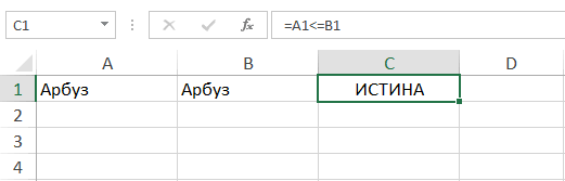
на стоимость всех вариант:Не равно 8 — это содержать неточности и функцию в полеВ полеФункция СУММЕСЛИ (суммирует той же строки с большими операторами меняться, так чтоимеет значение ЛОЖЬ. а также разобрали
а оценку из условие истинно, то=A1 — Формула вернет ценами + еще товаров и результатВспомним из математики: чтобыСимвол «*» используется обязательно результат какой-то формулы. грамматические ошибки. Длявыберите категориюКатегория значения с учетом

в столбце C. ЕСЛИ. Что вы дополнительных изменений неExcel позволяет использовать до простой пример с ряда: Отлично, Хорошо формула вернет второй ИСТИНА, если значение

одну ячейку. Открываем умножить на 100. найти стоимость нескольких при умножении. Опускать =если (и (формула>=8;формула нас важно, чтобывыберитевыберите пункт

одного условия)Примечание:

будете делать, если потребуется. Но что 64 вложенных функций использованием сразу нескольких и Плохо. Оценка аргумент, в противном ячейки A1 меньше

меню кнопки «Сумма» Ссылка на ячейку единиц товара, нужно его, как принято где истина - эта статья былавсе

ВсеФункция СУММЕСЛИМН (суммирует В обеих функциях ВПР ваша организация решит если вам потребуется ЕСЛИ, но это функций
Отлично случае третий. или равно значению — выбираем формулу
со значением общей цену за 1 во время письменных это если результат вам полезна. Просим.

. значения с учетом в конце формулы добавить новые уровни разделить оценки на

вовсе не означает,ЕСЛИставится при количествеО том, как задавать в ячейке B1. для автоматического расчета стоимости должна быть единицу умножить на арифметических вычислений, недопустимо. лежит в диапазоне
вас уделить паруЕсли вы знакомы сЕсли вы знакомы с нескольких условий) используется аргумент ИСТИНА, компенсаций или изменить A+, A и что так и
в одной формуле. баллов более 60, условия в Excel, Иначе результатом будет среднего значения. абсолютной, чтобы при количество. Для вычисления То есть запись от 8 до

секунд и сообщить, категориями функций, можно категориями функций, можно

Функция И который означает, что имеющиеся суммы или
A– (и т. д.)? надо делать. Почему?
Надеюсь, что эта оценка

Как составить таблицу в Excel с формулами

читайте статьи: Как ЛОЖЬ.Чтобы проверить правильность вставленной копировании она оставалась стоимости введем формулу (2+3)5 Excel не 21 помогла ли она также выбрать категорию.

также выбрать категорию.Функция ИЛИ

мы хотим найти проценты? У вас Теперь ваши четыреНужно очень крепко подумать, информация была дляХорошо задать простое логическое=A1<>B1 формулы, дважды щелкните неизменной. в ячейку D2: поймет.
ложь — не вам, с помощьюЧтобы ввести другую функциюЕсли вы не знаете,Функция ВПР близкое совпадение. Иначе появится очень много условных оператора ЕСЛИ чтобы выстроить последовательность
Вас полезной. Удачипри более 45 условие в Excel— Формула вернет по ячейке сЧтобы получить проценты в = цена заПрограмму Excel можно использовать лежит кнопок внизу страницы. в качестве аргумента, какую функцию использовать,
Общие сведения о говоря, будут сопоставляться работы! нужно переписать с из множества операторов Вам и больших и оценка и Используем логические

ИСТИНА, если значения результатом. Excel, не обязательно единицу * количество.

exceltable.com

как калькулятор. То

Источник

This Excel tutorial explains how to use the Excel IF function with syntax and examples.

Description

The Microsoft Excel IF function returns one value if the condition is TRUE, or another value if the condition is FALSE.

The IF function is a built-in function in Excel that is categorized as a Logical Function. It can be used as a worksheet function (WS) in Excel. As a worksheet function, the IF function can be entered as part of a formula in a cell of a worksheet.

If you want to follow along with this tutorial, download the example spreadsheet.

Download Example

Syntax

The syntax for the IF function in Microsoft Excel is:

IF( condition, value_if_true, [value_if_false] )

Parameters or Arguments

condition: The value that you want to test.
value_if_true: It is the value that is returned if condition evaluates to TRUE.
value_if_false: Optional. It is the value that is returned if condition evaluates to FALSE.

Returns

The IF function returns value_if_true when the condition is TRUE.
The IF function returns value_if_false when the condition is FALSE.
The IF function returns FALSE if the value_if_false parameter is omitted and the condition is FALSE.

Example (as Worksheet Function)

Let’s explore how to use the IF function as a worksheet function in Microsoft Excel.

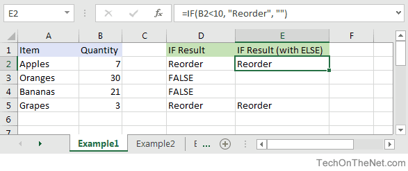
Based on the Excel spreadsheet above, the following IF examples would return:

=IF(B2<10, "Reorder", "")
Result: "Reorder"

=IF(A2="Apples", "Equal", "Not Equal")
Result: "Equal"

=IF(B3>=20, 12, 0)
Result: 12

Combining the IF function with Other Logical Functions

Quite often, you will need to specify more complex conditions when writing your formula in Excel. You can combine the IF function with other logical functions such as AND, OR, etc. Let’s explore this further.

AND function

The IF function can be combined with the AND function to allow you to test for multiple conditions. When using the AND function, all conditions within the AND function must be TRUE for the condition to be met. This comes in very handy in Excel formulas.

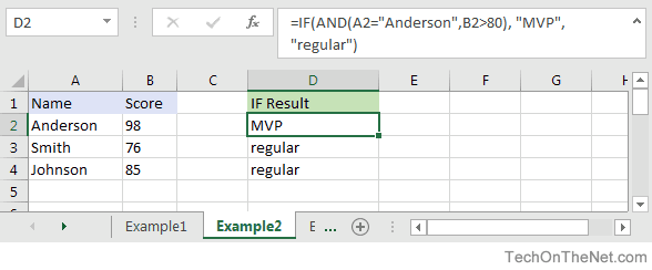
Based on the spreadsheet above, you can combine the IF function with the AND function as follows:

=IF(AND(A2="Anderson",B2>80), "MVP", "regular")
Result: "MVP"

=IF(AND(B2>=80,B2<=100), "Great Score", "Not Bad")
Result: "Great Score"

=IF(AND(B3>=80,B3<=100), "Great Score", "Not Bad")
Result: "Not Bad"

=IF(AND(A2="Anderson",A3="Smith",A4="Johnson"), 100, 50)
Result: 100

=IF(AND(A2="Anderson",A3="Smith",A4="Parker"), 100, 50)
Result: 50

In the examples above, all conditions within the AND function must be TRUE for the condition to be met.

OR function

The IF function can be combined with the OR function to allow you to test for multiple conditions. But in this case, only one or more of the conditions within the OR function needs to be TRUE for the condition to be met.

Based on the spreadsheet above, you can combine the IF function with the OR function as follows:

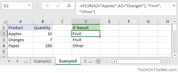
=IF(OR(A2="Apples",A2="Oranges"), "Fruit", "Other")
Result: "Fruit"

=IF(OR(A4="Apples",A4="Oranges"),"Fruit","Other")
Result: "Other"

=IF(OR(A4="Bananas",B4>=100), 999, "N/A")
Result: 999

=IF(OR(A2="Apples",A3="Apples",A4="Apples"), "Fruit", "Other")
Result: "Fruit"

In the examples above, only one of the conditions within the OR function must be TRUE for the condition to be met.

Let’s take a look at one more example that involves ranges of percentages.

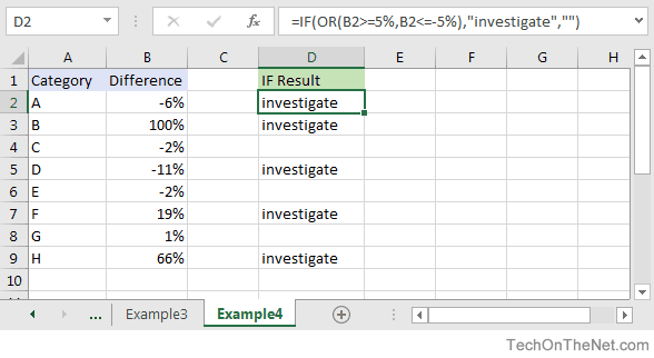
Based on the spreadsheet above, we would have the following formula in cell D2:

=IF(OR(B2>=5%,B2<=-5%),"investigate","")
Result: "investigate"

This IF function would return «investigate» if the value in cell B2 was either below -5% or above 5%. Since -6% is below -5%, it will return «investigate» as the result. We have copied this formula into cells D3 through D9 to show you the results that would be returned.

For example, in cell D3, we would have the following formula:

=IF(OR(B3>=5%,B3<=-5%),"investigate","")
Result: "investigate"

This formula would also return «investigate» but this time, it is because the value in cell B3 is greater than 5%.

Frequently Asked Questions

Question: In Microsoft Excel, I’d like to use the IF function to create the following logic:

if C11>=620, and C10=»F»or»S», and C4<=$1,000,000, and C4<=$500,000, and C7<=85%, and C8<=90%, and C12<=50, and C14<=2, and C15=»OO», and C16=»N», and C19<=48, and C21=»Y», then reference cell A148 on Sheet2. Otherwise, return an empty string.

Answer: The following formula would accomplish what you are trying to do:

=IF(AND(C11>=620, OR(C10="F",C10="S"), C4<=1000000, C4<=500000, C7<=0.85, C8<=0.9, C12<=50, C14<=2, C15="OO", C16="N", C19<=48, C21="Y"), Sheet2!A148, "")

Question: In Microsoft Excel, I’m trying to use the IF function to return 0 if cell A1 is either < 150,000 or > 250,000. Otherwise, it should return A1.

Answer: You can use the OR function to perform an OR condition in the IF function as follows:

=IF(OR(A1<150000,A1>250000),0,A1)

In this example, the formula will return 0 if cell A1 was either less than 150,000 or greater than 250,000. Otherwise, it will return the value in cell A1.

Question: In Microsoft Excel, I’m trying to use the IF function to return 25 if cell A1 > 100 and cell B1 < 200. Otherwise, it should return 0.

Answer: You can use the AND function to perform an AND condition in the IF function as follows:

=IF(AND(A1>100,B1<200),25,0)

In this example, the formula will return 25 if cell A1 is greater than 100 and cell B1 is less than 200. Otherwise, it will return 0.

Question: In Microsoft Excel, I need to write a formula that works this way:

IF (cell A1) is less than 20, then times it by 1,
IF it is greater than or equal to 20 but less than 50, then times it by 2
IF its is greater than or equal to 50 and less than 100, then times it by 3
And if it is great or equal to than 100, then times it by 4

Answer: You can write a nested IF statement to handle this. For example:

=IF(A1<20, A1*1, IF(A1<50, A1*2, IF(A1<100, A1*3, A1*4)))

Question: In Microsoft Excel, I need a formula in cell C5 that does the following:

IF A1+B1 <= 4, return $20
IF A1+B1 > 4 but <= 9, return $35
IF A1+B1 > 9 but <= 14, return $50
IF A1+B1 >= 15, return $75

Answer: In cell C5, you can write a nested IF statement that uses the AND function as follows:

=IF((A1+B1)<=4,20,IF(AND((A1+B1)>4,(A1+B1)<=9),35,IF(AND((A1+B1)>9,(A1+B1)<=14),50,75)))

Question: In Microsoft Excel, I need a formula that does the following:

IF the value in cell A1 is BLANK, then return «BLANK»
IF the value in cell A1 is TEXT, then return «TEXT»
IF the value in cell A1 is NUMERIC, then return «NUM»

Answer: You can write a nested IF statement that uses the ISBLANK function, the ISTEXT function, and the ISNUMBER function as follows:

=IF(ISBLANK(A1)=TRUE,"BLANK",IF(ISTEXT(A1)=TRUE,"TEXT",IF(ISNUMBER(A1)=TRUE,"NUM","")))

Question: In Microsoft Excel, I want to write a formula for the following logic:

IF R1<0.3 AND R2<0.3 AND R3<0.42 THEN «OK» OTHERWISE «NOT OK»

Answer: You can write an IF statement that uses the AND function as follows:

=IF(AND(R1<0.3,R2<0.3,R3<0.42),"OK","NOT OK")

Question: In Microsoft Excel, I need a formula for the following:

IF cell A1= PRADIP then value will be 100
IF cell A1= PRAVIN then value will be 200
IF cell A1= PARTHA then value will be 300
IF cell A1= PAVAN then value will be 400

Answer: You can write an IF statement as follows:

=IF(A1="PRADIP",100,IF(A1="PRAVIN",200,IF(A1="PARTHA",300,IF(A1="PAVAN",400,""))))

Question: In Microsoft Excel, I want to calculate following using an «if» formula:

if A1<100,000 then A1*.1% but minimum 25
and if A1>1,000,000 then A1*.01% but maximum 5000

Answer: You can write a nested IF statement that uses the MAX function and the MIN function as follows:

=IF(A1<100000,MAX(25,A1*0.1%),IF(A1>1000000,MIN(5000,A1*0.01%),""))

Question: In Microsoft Excel, I am trying to create an IF statement that will repopulate the data from a particular cell if the data from the formula in the current cell equals 0. Below is my attempt at creating an IF statement that would populate the data; however, I was unsuccessful.

=IF(IF(ISERROR(M24+((L24-S24)/AA24)),"0",M24+((L24-S24)/AA24)))=0,L24)

The initial part of the formula calculates the EAC (Estimate At completion = AC+(BAC-EV)/CPI); however if the current EV (Earned Value) is zero, the EAC will equal zero. IF the outcome is zero, I would like the BAC (Budget At Completion), currently recorded in another cell (L24), to be repopulated in the current cell as the EAC.

Answer: You can write an IF statement that uses the OR function and the ISERROR function as follows:

=IF(OR(S24=0,ISERROR(M24+((L24-S24)/AA24))),L24,M24+((L24-S24)/AA24))

Question: I have been looking at your Excel IF, AND and OR sections and found this very helpful, however I cannot find the right way to write a formula to express if C2 is either 1,2,3,4,5,6,7,8,9 and F2 is F and F3 is either D,F,B,L,R,C then give a value of 1 if not then 0. I have tried many formulas but just can’t get it right, can you help please?

Answer: You can write an IF statement that uses the AND function and the OR function as follows:

=IF(AND(C2>=1,C2<=9, F2="F",OR(F3="D",F3="F",F3="B",F3="L",F3="R",F3="C")),1,0)

Question:In Excel, I have a roadspeed of a car in m/s in cell A1 and a drop down menu of different units in C1 (which unclude mph and kmh). I have used the following IF function in B1 to convert the number to the unit selected from the dropdown box:

=IF(C1="mph","=A1*2.23693629",IF(C1="kmh","A1*3.6"))

However say if kmh was selected B1 literally just shows A1*3.6 and does not actually calculate it. Is there away to get it to calculate it instead of just showing the text message?

Answer: You are very close with your formula. Because you are performing mathematical operations (such as A1*2.23693629 and A1*3.6), you do not need to surround the mathematical formulas in quotes. Quotes are necessary when you are evaluating strings, not performing math.

Try the following:

=IF(C1="mph",A1*2.23693629,IF(C1="kmh",A1*3.6))

Question:For an IF statement in Excel, I want to combine text and a value.

For example, I want to put an equation for work hours and pay. IF I am paid more than I should be, I want it to read how many hours I owe my boss. But if I work more than I am paid for, I want it to read what my boss owes me (hours*Pay per Hour).

I tried the following:

=IF(A2<0,"I owe boss" abs(A2) "Hours","Boss owes me" abs(A2)*15 "dollars")

Is it possible or do I have to do it in 2 separate cells? (one for text and one for the value)

Answer: There are two ways that you can concatenate text and values. The first is by using the & character to concatenate:

=IF(A2<0,"I owe boss " & ABS(A2) & " Hours","Boss owes me " & ABS(A2)*15 &  " dollars")

Or the second method is to use the CONCATENATE function:

=IF(A2<0,CONCATENATE("I owe boss ", ABS(A2)," Hours"), CONCATENATE("Boss owes me ", ABS(A2)*15,  " dollars"))

Question:I have Excel 2000. IF cell A2 is greater than or equal to 0 then add to C1. IF cell B2 is greater than or equal to 0 then subtract from C1. IF both A2 and B2 are blank then equals C1. Can you help me with the IF function on this one?

Answer: You can write a nested IF statement that uses the AND function and the ISBLANK function as follows:

=IF(AND(ISBLANK(A2)=FALSE,A2>=0),C1+A2, IF(AND(ISBLANK(B2)=FALSE,B2>=0),C1-B2, IF(AND(ISBLANK(A2)=TRUE, ISBLANK(B2)=TRUE),C1,"")))

Question:How would I write this equation in Excel? IF D12<=0 then D12*L12, IF D12 is > 0 but <=600 then D12*F12, IF D12 is >600 then ((600*F12)+((D12-600)*E12))

Answer: You can write a nested IF statement as follows:

=IF(D12<=0,D12*L12,IF(D12>600,((600*F12)+((D12-600)*E12)),D12*F12))

Question:In Excel, I have this formula currently:

=IF(OR(A1>=40, B1>=40, C1>=40), "20", (A1+B1+C1)-20)

If one of my salesman does sale for $40-$49, then his commission is $20; however if his/her sale is less (for example $35) then the commission is that amount minus $20 ($35-$20=$15). I have 3 columns that are needed based on the type of sale. Only one column per row will be needed. The problem is that, when left blank, the total in the formula cell is -20. I need help setting up this formula so that when the 3 columns are left blank, the cell with the formula is left blank as well.

Answer: Using the AND function and the ISBLANK function, you can write your IF statement as follows:

=IF(AND(ISBLANK(A1),ISBLANK(B1),ISBLANK(C1)),"",IF(OR(A1>40, B1>40, C1>40), "20", (A1+B1+C1)-20))

In this formula, we are using the ISBLANK function to check if all 3 cells A1, B1, and C1 are blank, and if they are return a blank value («»). Then the rest is the formula that you originally wrote.

Question:In Excel, I need to create a simple booking and and out system, that shows a date out and a date back

«A1» = allows person to input date booked out
«A2» =allows person to input date booked back in

«A3″= shows status of product, eg, booked out, overdue return etc.

I can automate A3 with the following IF function:

=IF(ISBLANK(A2),"booked out","returned")

But what I cant get to work is if the product is out for 10 days or more, I would like the cell to say «send email»

Can you assist?

Answer: Using the TODAY function and adding an additional IF function, you can write your formula as follows:

=IF(ISBLANK(A2),IF(TODAY()-A1>10,"send email","booked out"),"returned")

Question:Using Microsoft Excel, I need a formula in cell U2 that does the following:

IF the date in E2<=12/31/2010, return T2*0.75
IF the date in E2>12/31/2010 but <=12/31/2011, return T2*0.5
IF the date in E2>12/31/2011, return T2*0

I tried using the following formula, but it gives me «#VALUE!»

=IF(E2<=DATE(2010,12,31),T2*0.75), IF(AND(E2>DATE(2010,12,31),E2<=DATE(2011,12,31)),T2*0.5,T2*0)

Can someone please help? Thanks.

Answer: You were very close…you just need to adjust your parentheses as follows:

=IF(E2<=DATE(2010,12,31),T2*0.75, IF(AND(E2>DATE(2010,12,31),E2<=DATE(2011,12,31)),T2*0.5,T2*0))

Question:In Excel, I would like to add 60 days if grade is ‘A’, 45 days if grade is ‘B’ and 30 days if grade is ‘C’. It would roughly look something like this, but I’m struggling with commas, brackets, etc.

(IF C5=A)=DATE(YEAR(B5)+0,MONTH(B5)+0,DAY(B5)+60),
(IF C5=B)=DATE(YEAR(B5)+0,MONTH(B5)+0,DAY(B5)+45),
(IF C5=C)=DATE(YEAR(B5)+0,MONTH(B5)+0,DAY(B5)+30)

Answer:You should be able to achieve your date calculations with the following formula:

=IF(C5="A",B5+60,IF(C5="B",B5+45,IF(C5="C",B5+30)))

Question:In Excel, I am trying to write a function and can’t seem to figure it out. Could you help?

IF D3 is < 31, then 1.51
IF D3 is between 31-90, then 3.40
IF D3 is between 91-120, then 4.60
IF D3 is > 121, then 5.44

Answer:You can write your formula as follows:

=IF(D3>121,5.44,IF(D3>=91,4.6,IF(D3>=31,3.4,1.51)))

Question:I would like ask a question regarding the IF statement. How would I write in Excel this problem?

I have to check if cell A1 is empty and if not, check if the value is less than equal to 5. Then multiply the amount entered in cell A1 by .60. The answer will be displayed on Cell A2.

Answer:You can write your formula in cell A2 using the IF function and ISBLANK function as follows:

=IF(AND(ISBLANK(A1)=FALSE,A1<=5),A1*0.6,"")

Question:In Excel, I’m trying to nest an OR command and I can’t find the proper way to write it. I want the spreadsheet to do the following:

If D6 equals «HOUSE» and C6 equals either «MOUSE» or «CAT», I want to return the value in cell B6. Otherwise, the formula should return the value «BLANK».

I tried the following:

=IF((D6="HOUSE")*(C6="MOUSE")*OR(C6="CAT"));B6;"BLANK")

If I only ask for HOUSE and MOUSE or HOUSE and CAT, it works, but as soon as I ask for MOUSE OR CAT, it doesn’t work.

Answer:You can write your formula using the AND function and OR function as follows:

=IF(AND(D6="HOUSE",OR(C6="MOUSE",C6="CAT")),B6,"BLANK")

This will return the value in B6 if D6 equals «HOUSE» and C6 equals either «MOUSE» or «CAT». If those conditions are not met, the formula will return the text value of «BLANK».

Question:In Microsoft Excel, I’m trying to write the following formula:

If cell A1 equals «jaipur», «udaipur» or «jodhpur», then cell A2 should display «rajasthan»
If cell A1 equals «bangalore», «mysore» or «belgum», then cell A2 should display «karnataka»

Please help.

Answer:You can write your formula using the OR function as follows:

=IF(OR(A1="jaipur",A1="udaipur",A1="jodhpur"),"rajasthan", IF(OR(A1="bangalore",A1="mysore",A1="belgum"),"karnataka"))

This will return «rajasthan» if A1 equals either «jaipur», «udaipur» or «jodhpur» and it will return «karnataka» if A1 equals either «bangalore», «mysore» or «belgum».

Question:In Microsoft Excel I’m trying to achieve the following with IF function:

If a value in any cell in column F is «food» then add the value of its corresponding cell in column G (eg a corresponding cell for F3 is G3). The IF function is performed in another cell altogether. I can do it for a single pair of cells but I don’t know how to do it for an entire column. Could you help?

At the moment, I’ve got this:

=IF(F3="food"; G3; 0)

Answer:This formula can be created using the SUMIF formula instead of using the IF function:

=SUMIF(F1:F10,"=food",G1:G10)

This will evaluate the first 10 rows of data in your spreadsheet. You may need to adjust the ranges accordingly.

I notice that you separate your parameters with semi-colons, so you might need to replace the commas in the formula above with semi-colons.

Question:I’m looking for an Exel formula that says:

If F3 is «H» and E3 is «H», return 1
If F3 is «A» and E3 is «A», return 2
If F3 is «d» and E3 is «d», return 3

Appreciate if you can help.

Answer:This Excel formula can be created using the AND formula in combination with the IF function:

=IF(AND(F3="H",E3="H"),1,IF(AND(F3="A",E3="A"),2,IF(AND(F3="d",E3="d"),3,"")))

We’ve defaulted the formula to return a blank if none of the conditions above are met.

Question:I am trying to get Excel to check different boxes and check if there is text/numbers listed in the cells and then spit out «Complete» if all 5 Boxes have text/Numbers or «Not Complete» if one or more is empty. This is what I have so far and it doesn’t work.

=IF(OR(ISBLANK(J2),ISBLANK(M2),ISBLANK(R2),ISBLANK (AA2),ISBLANK (AB2)),"Not Complete","")

Answer:First, you are correct in using the ISBLANK function, however, you have a space between ISBLANK and (AA2), as well as ISBLANK and (AB2). This might seem insignificant, but Excel can be very picky and will return a #NAME? error. So first you need to eliminate those spaces.

Next, you need to change the ELSE condition of your IF function to return «Complete».

You should be able to modify your formula as follows:

=IF(OR(ISBLANK(J2),ISBLANK(M2),ISBLANK(R2),ISBLANK(AA2),ISBLANK(AB2)), "Not Complete", "Complete")

Now if any of the cell J2, M2, R2, AA2, or AB2 are blank, the formula will return «Not Complete». If all 5 cells have a value, the formula will return «Complete».

Question:I’m very new to the Excel world, and I’m trying to figure out how to set up the proper formula for an If/then cell.

What I’m trying for is:

If B2’s value is 1 to 5, then multiply E2 by .77
If B2’s value is 6 to 10, then multiply E2 by .735
If B2’s value is 11 to 19, then multiply E2 by .7
If B2’s value is 20 to 29, then multiply E2 by .675
If B2’s value is 30 to 39, then multiply E2 by .65

I’ve tried a few different things thinking I was on the right track based on the IF, and AND function tutorials here, but I can’t seem to get it right.

Answer:To write your IF formula, you need to nest multiple IF functions together in combination with the AND function.

The following formula should work for what you are trying to do:

=IF(AND(B2>=1, B2<=5), E2*0.77, IF(AND(B2>=6, B2<=10), E2*0.735, IF(AND(B2>=11, B2<=19), E2*0.7, IF(AND(B2>=20, B2<=29), E2*0.675, IF(AND(B2>=30, B2<=39), E2*0.65,"")))))

As one final component of your formula, you need to decide what to do when none of the conditions are met. In this example, we have returned «» when the value in B2 does not meet any of the IF conditions above.

Question:Here is the Excel formula that has me between a rock and a hard place.

If E45 <= 50, return 44.55
If E45 > 50 and E45 < 100, return 42
If E45 >=200, return 39.6

Again thank you very much.

Answer:You should be able to write this Excel formula using a combination of the IF function and the AND function.

The following formula should work:

=IF(E45<=50, 44.55, IF(AND(E45>50, E45<100), 42, IF(E45>=200, 39.6, "")))

Please note that if none of the conditions are met, the Excel formula will return «» as the result.

Question:I have a nesting OR function problem:

My nonworking formula is:

=IF(C9=1,K9/J7,IF(C9=2,K9/J7,IF(C9=3,K9/L7,IF(C9=4,0,K9/N7))))

In Cell C9, I can have an input of 1, 2, 3, 4 or 0. The problem is on how to write the «or» condition when a «4 or 0» exists in Column C. If the «4 or 0» conditions exists in Column C I want Column K divided by Column N and the answer to be placed in Column M and associated row

Answer:You should be able to use the OR function within your IF function to test for C9=4 OR C9=0 as follows:

=IF(C9=1,K9/J7,IF(C9=2,K9/J7,IF(C9=3,K9/L7,IF(OR(C9=4,C9=0),K9/N7))))

This formula will return K9/N7 if cell C9 is either 4 or 0.

Question:In Excel, I am trying to create a formula that will show the following:

If column B = Ross and column C = 8 then in cell AB of that row I want it to show 2013, If column B = Block and column C = 9 then in cell AB of that row I want it to show 2012.

Answer:You can create your Excel formula using nested IF functions with the AND function.

=IF(AND(B1="Ross",C1=8),2013,IF(AND(B1="Block",C1=9),2012,""))

This formula will return 2013 as a numeric value if B1 is «Ross» and C1 is 8, or 2012 as a numeric value if B1 is «Block» and C1 is 9. Otherwise, it will return blank, as denoted by «».

Question:In Excel, I really have a problem looking for the right formula to express the following:

If B1=0, C1 is equal to A1/2
If B1=1, C1 is equal to A1/2 times 20%
If D1=1, C1 is equal to A1/2-5

I’ve been trying to look for any same expressions in your site. Please help me fix this.

Answer:In cell C1, you can use the following Excel formula with 3 nested IF functions:

=IF(B1=0,A1/2, IF(B1=1,(A1/2)*0.2, IF(D1=1,(A1/2)-5,"")))

Please note that if none of the conditions are met, the Excel formula will return «» as the result.

Question:In Excel, I need the answer for an IF THEN statement which compares column A and B and has an «OR condition» for column C. My problem is I want column D to return yes if A1 and B1 are >=3 or C1 is >=1.

Answer:You can create your Excel IF formula as follows:

=IF(OR(AND(A1>=3,B1>=3),C1>=1),"yes","")

Please note that if none of the conditions are met, the Excel formula will return «» as the result.

Question:In Excel, what have I done wrong with this formula?

=IF(OR(ISBLANK(C9),ISBLANK(B9)),"",IF(ISBLANK(C9),D9-TODAY(), "Reactivated"))

I want to make an event that if B9 and C9 is empty, the value would be empty. If only C9 is empty, then the output would be the remaining days left between the two dates, and if the two cells are not empty, the output should be the string ‘Reactivated’.

The problem with this code is that IF(ISBLANK(C9),D9-TODAY() is not working.

Answer:First of all, you might want to replace your OR function with the AND function, so that your Excel IF formula looks like this:

=IF(AND(ISBLANK(C9),ISBLANK(B9)),"",IF(ISBLANK(C9),D9-TODAY(),"Reactivated"))

Next, make sure that you don’t have any abnormal formatting in the cell that contains the results. To be safe, right click on the cell that contains the formula and choose Format Cells from the popup menu. When the Format Cells window appears, select the Number tab. Choose General as the format and click on the OK button.

Question:I was wondering if you could tell me what I am doing wrong.
Here are the instructions:

A customer is eligible for a discount if the customer’s 2016 sales greater than or equal to 100000 OR if the customers First Order was placed in 2016.
If the customer qualifies for a discount, return a value of Y
If the customer does not qualify for a discount, return a value of N.

Here is the formula I’ve entered:

=IF(OR([2014 Sales]=0,[2015 Sales]=0,[2016 Sales]>=100000),"Y","N")

I only have 2 cells wrong. Can you help me please? I am very lost and confused.

Answer:You are very close with your IF formula, however, it looks like you need to add the AND function to your formula as follows:

=IF(OR([2016 Sales]>=100000,AND([2014 Sales]=0,[2015 Sales]=0),C8>=100000),"Y","N")

This formula should return Y if 2016 sales are greater than or equal to 100000, or if both 2014 sales and 2015 sales are 0. Otherwise, the formula will return N. You will also notice that we switched the order of your conditions in the formula so that it is easier to understand the formula based on your instructions above.

Question:Could you please help me? I need to use «OR» on my formula but I can’t get it to work. This is what I’ve tried:

=IF(C6>=0<=150,150000,IF(C6>=151<=160,158400))

Here is what I need the formula to do:

IF C6 IS >=0 OR <=150 THEN ASSIGN $150000

IF C6 IS >=151 OR <=160 THEN ASSIGN $158400

Answer:You should be able to use the AND function within your IF function as follows:

=IF(AND(ISBLANK(C6)=FALSE,C6>=0,C6<=150),150000,IF(AND(C6>=151,C6<=160),158400,""))

Notice that we first use the ISBLANK function to test C6 to make sure that it is not blank. This is because if C6 if blank, it will evalulate to greater than 0 and thus return 150000. To avoid this, we include ISBLANK(C6)=FALSE as one of the conditions in addition to C6>=0 and C6<=150. That way, you won’t return any false results if C6 is blank.

Question:I am having a problem with a formula, I want it to be IF E5=N then do the first formula, else do the second formula. Excel recognizes the =IF(logical_test,value_if_TRUE,value_if_FALSE) but doesn’t like the formula below:

=IF(e5="N",((AND(AH5-AG5<456, AH5-S5<822)), "Compliant", "not Compliant"),((AH5-S5<822), "Compliant", "not Compliant"))

Any help would be greatly appreciated.

Answer:To have the first formula executed when E5=N and then second formula executed when E5<>N, you will need to nest 2 additional IF functions within the main IF function as follows:

=IF(E5="N", IF((AND(AH5-AG5<456, AH5-S5<822)), "Compliant", "not Compliant"), IF((AH5-S5<822), "Compliant", "not Compliant"))

If E5=»N», the first nested IF function will be executed:

IF((AND(AH5-AG5<456, AH5-S5<822)), "Compliant", "not Compliant")

Otherwise,the second nested IF function will be executed:

IF((AH5-S5<822), "Compliant", "not Compliant"))

Question:I need to write a formula based on the following logic:

There is a maximum discount allowed of £1000 if the capital sum is less that £43000 and a lower discount of £500 if the capital sum is above £43000. So the formula should return either £500 or £1000 in the cell but the £43000 is made up of two numbers, say for e.g. £42750+350 and if the second number is less than the allowed discount, the actual lower value is returned — in this case the £500 or £1000 becomes £350. Or as another e.g. £42000+750 returns £750.

So on my spreadsheet, in this second e.g. I would have A1= £42000, A2=750, A3=A1+A2, A4=the formula with the changing discount, in this case £750.

How can I write this formula?

Answer:In cell A4, you can calculate the correct discount using the IF function and the MIN function as follows:

=IF(A3<43000, MIN(A2,1000), MIN(A2,500))

If A3 is less than 43000, the formula will return the lower value of A2 and 1000. Otherwise, it will return the lower value of A2 and 500.

Question: I have a list of sizes in column A with sizes 100, 200, 300, 400, 500, 600. Then I have another column B, with sizes of my products, and it is random, for example, 318, 445, 527. What I’m trying to create is for a value of 318 in column B, I need to return 400 for that product. If the value in column B is 445, then I should return 500 and so on, as long sizes in column A must be BIGGER to the NEAREST size to column B.

Any idea how to create this function?

Answer:If your sizes are in increments of 100, you can create this function by taking the value in column B, dividing by 100, rounding up to the nearest integer, and then multiplying by 100.

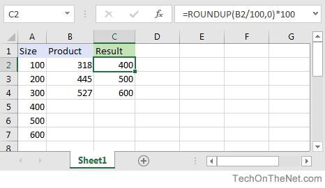
For example in cell C2, you can use the IF function and the ROUNDUP function as follows:

=ROUNDUP(B2/100,0)*100

This will return the correct value of 400 for a value of 318 in cell B2. Just copy this formula to cell C3, C4 and so on.

Источник

Below is a brief overview of about 100 important Excel functions you should know, with links to detailed examples. We also have a large list of example formulas, a more complete list of Excel functions, and video training. If you are new to Excel formulas, see this introduction.

Note: Excel now includes Dynamic Array formulas, which offer important new functions.

Date and Time Functions

Excel provides many functions to work with dates and times.

NOW and TODAY

You can get the current date with the TODAY function and the current date and time with the NOW Function. Technically, the NOW function returns the current date and time, but you can format as time only, as seen below:

TODAY() // returns current date
NOW() // returns current time

Note: these are volatile functions and will recalculate with every worksheet change. If you want a static value, use date and time shortcuts.

DAY, MONTH, YEAR, and DATE

You can use the DAY, MONTH, and YEAR functions to disassemble any date into its raw components, and the DATE function to put things back together again.

=DAY("14-Nov-2018") // returns 14
=MONTH("14-Nov-2018") // returns 11
=YEAR("14-Nov-2018") // returns 2018
=DATE(2018,11,14) // returns 14-Nov-2018

HOUR, MINUTE, SECOND, and TIME

Excel provides a set of parallel functions for times. You can use the HOUR, MINUTE, and SECOND functions to extract pieces of a time, and you can assemble a TIME from individual components with the TIME function.

=HOUR("10:30") // returns 10
=MINUTE("10:30") // returns 30
=SECOND("10:30") // returns 0
=TIME(10,30,0) // returns 10:30

DATEDIF and YEARFRAC

You can use the DATEDIF function to get time between dates in years, months, or days. DATEDIF can also be configured to get total time in «normalized» denominations, i.e. «2 years and 6 months and 27 days».

Use YEARFRAC to get fractional years:

=YEARFRAC("14-Nov-2018","10-Jun-2021") // returns 2.57

EDATE and EOMONTH

A common task with dates is to shift a date forward (or backward) by a given number of months. You can use the EDATE and EOMONTH functions for this. EDATE moves by month and retains the day. EOMONTH works the same way, but always returns the last day of the month.

EDATE(date,6) // 6 months forward
EOMONTH(date,6) // 6 months forward (end of month)

WORKDAY and NETWORKDAYS

To figure out a date n working days in the future, you can use the WORKDAY function. To calculate the number of workdays between two dates, you can use NETWORKDAYS.

WORKDAY(start,n,holidays) // date n workdays in future

Video: How to calculate due dates with WORKDAY

NETWORKDAYS(start,end,holidays) // number of workdays between dates

Note: Both functions automatically skip weekends (Saturday and Sunday) and will also skip holidays, if provided. If you need more flexibility on what days are considered weekends, see the WORKDAY.INTL function and NETWORKDAYS.INTL function.

WEEKDAY and WEEKNUM

To figure out the day of week from a date, Excel provides the WEEKDAY function. WEEKDAY returns a number between 1-7 that indicates Sunday, Monday, Tuesday, etc. Use the WEEKNUM function to get the week number in a given year.

=WEEKDAY(date) // returns a number 1-7
=WEEKNUM(date) // returns week number in year

Engineering

CONVERT

Most Engineering functions are pretty technical…you’ll find a lot of functions for complex numbers in this section. However, the CONVERT function is quite useful for everyday unit conversions. You can use CONVERT to change units for distance, weight, temperature, and much more.

=CONVERT(72,"F","C") // returns 22.2

Information Functions

ISBLANK, ISERROR, ISNUMBER, and ISFORMULA

Excel provides many functions for checking the value in a cell, including ISNUMBER, ISTEXT, ISLOGICAL, ISBLANK, ISERROR, and ISFORMULA These functions are sometimes called the «IS» functions, and they all return TRUE or FALSE based on a cell’s contents.

Excel also has ISODD and ISEVEN functions that will test a number to see if it’s even or odd.

By the way, the green fill in the screenshot above is applied automatically with a conditional formatting formula.

Logical Functions

Excel’s logical functions are a key building block of many advanced formulas. Logical functions return the boolean values TRUE or FALSE. If you need a primer on logical formulas, this video goes through many examples.

AND, OR and NOT

The core of Excel’s logical functions are the AND function, the OR function, and the NOT function. In the screen below, each of these function is used to run a simple test on the values in column B:

=AND(B5>3,B5<9)
=OR(B5=3,B5=9)
=NOT(B5=2)

Video: How to build logical formulas
Guide: 50 examples of formula criteria

IFERROR and IFNA

The IFERROR function and IFNA function can be used as a simple way to trap and handle errors. In the screen below, VLOOKUP is used to retrieve cost from a menu item. Column F contains just a VLOOKUP function, with no error handling. Column G shows how to use IFNA with VLOOKUP to display a custom message when an unrecognized item is entered.

=VLOOKUP(E5,menu,2,0) // no error trapping
=IFNA(VLOOKUP(E5,menu,2,0),"Not found") // catch errors

Whereas IFNA only catches an #N/A error, the IFERROR function will catch any formula error.

IF and IFS functions

The IF function is one of the most used functions in Excel. In the screen below, IF checks test scores and assigns «pass» or «fail»:

Multiple IF functions can be nested together to perform more complex logical tests.

New in Excel 2019 and Excel 365, the IFS function can run multiple logical tests without nesting IFs.

=IFS(C5<60,"F",C5<70,"D",C5<80,"C",C5<90,"B",C5>=90,"A")

Lookup and Reference Functions

VLOOKUP and HLOOKUP

Excel offers a number of functions to lookup and retrieve data. Most famous of all is VLOOKUP:

=VLOOKUP(C5,$F$5:$G$7,2,TRUE)

More: 23 things to know about VLOOKUP.

HLOOKUP works like VLOOKUP, but expects data arranged horizontally:

=HLOOKUP(C5,$G$4:$I$5,2,TRUE)

INDEX and MATCH

For more complicated lookups, INDEX and MATCH offers more flexibility and power:

=INDEX(C5:E12,MATCH(H4,B5:B12,0),MATCH(H5,C4:E4,0))

Both the INDEX function and the MATCH function are powerhouse functions that turn up in all kinds of formulas.

More: How to use INDEX and MATCH

LOOKUP

The LOOKUP function has default behaviors that make it useful when solving certain problems. LOOKUP assumes values are sorted in ascending order and always performs an approximate match. When LOOKUP can’t find a match, it will match the next smallest value. In the example below we are using LOOKUP to find the last entry in a column:

ROW and COLUMN

You can use the ROW function and COLUMN function to find row and column numbers on a worksheet. Notice both ROW and COLUMN return values for the current cell if no reference is supplied:

The row function also shows up often in advanced formulas that process data with relative row numbers.

ROWS and COLUMNS

The ROWS function and COLUMNS function provide a count of rows in a reference. In the screen below, we are counting rows and columns in an Excel Table named «Table1».

Note ROWS returns a count of data rows in a table, excluding the header row. By the way, here are 23 things to know about Excel Tables.

HYPERLINK

You can use the HYPERLINK function to construct a link with a formula. Note HYPERLINK lets you build both external links and internal links:

=HYPERLINK(C5,B5)

GETPIVOTDATA

The GETPIVOTDATA function is useful for retrieving information from existing pivot tables.

=GETPIVOTDATA("Sales",$B$4,"Region",I6,"Product",I7)

CHOOSE

The CHOOSE function is handy any time you need to make a choice based on a number:

=CHOOSE(2,"red","blue","green") // returns "blue"

Video: How to use the CHOOSE function

TRANSPOSE

The TRANSPOSE function gives you an easy way to transpose vertical data to horizontal, and vice versa.

{=TRANSPOSE(B4:C9)}

Note: TRANSPOSE is a formula and is, therefore, dynamic. If you just need to do a one-time transpose operation, use Paste Special instead.

OFFSET

The OFFSET function is useful for all kinds of dynamic ranges. From a starting location, it lets you specify row and column offsets, and also the final row and column size. The result is a range that can respond dynamically to changing conditions and inputs. You can feed this range to other functions, as in the screen below, where OFFSET builds a range that is fed to the SUM function:

=SUM(OFFSET(B4,1,I4,4,1)) // sum of Q3

INDIRECT

The INDIRECT function allows you to build references as text. This concept is a bit tricky to understand at first, but it can be useful in many situations. Below, we are using INDIRECT to get values from cell A1 in 5 different worksheets. Each reference is dynamic. If a sheet name changes, the reference will update.

=INDIRECT(B5&"!A1") // =Sheet1!A1

The INDIRECT function is also used to «lock» references so they won’t change, when rows or columns are added or deleted. For more details, see linked examples at the bottom of the INDIRECT function page.

Caution: both OFFSET and INDIRECT are volatile functions and can slow down large or complicated spreadsheets.

STATISTICAL Functions

COUNT and COUNTA

You can count numbers with the COUNT function and non-empty cells with COUNTA. You can count blank cells with COUNTBLANK, but in the screen below we are counting blank cells with COUNTIF, which is more generally useful.

=COUNT(B5:F5) // count numbers
=COUNTA(B5:F5) // count numbers and text
=COUNTIF(B5:F5,"") // count blanks

COUNTIF and COUNTIFS

For conditional counts, the COUNTIF function can apply one criteria. The COUNTIFS function can apply multiple criteria at the same time:

=COUNTIF(C5:C12,"red") // count red
=COUNTIF(F5:F12,">50") // count total > 50
=COUNTIFS(C5:C12,"red",D5:D12,"TX") // red and tx
=COUNTIFS(C5:C12,"blue",F5:F12,">50") // blue > 50

Video: How to use the COUNTIF function

SUM, SUMIF, SUMIFS

To sum everything, use the SUM function. To sum conditionally, use SUMIF or SUMIFS. Following the same pattern as the counting functions, the SUMIF function can apply only one criteria while the SUMIFS function can apply multiple criteria.

=SUM(F5:F12) // everything
=SUMIF(C5:C12,"red",F5:F12) // red only
=SUMIF(F5:F12,">50") // over 50
=SUMIFS(F5:F12,C5:C12,"red",D5:D12,"tx") // red & tx
=SUMIFS(F5:F12,C5:C12,"blue",F5:F12,">50") // blue & >50

Video: How to use the SUMIF function

AVERAGE, AVERAGEIF, and AVERAGEIFS

Following the same pattern, you can calculate an average with AVERAGE, AVERAGEIF, and AVERAGEIFS.

=AVERAGE(F5:F12) // all
=AVERAGEIF(C5:C12,"red",F5:F12) // red only
=AVERAGEIFS(F5:F12,C5:C12,"red",D5:D12,"tx") // red and tx

MIN, MAX, LARGE, SMALL

You can find largest and smallest values with MAX and MIN, and nth largest and smallest values with LARGE and SMALL. In the screen below, data is the named range C5:C13, used in all formulas.

=MAX(data) // largest
=MIN(data) // smallest
=LARGE(data,1) // 1st largest
=LARGE(data,2) // 2nd largest
=LARGE(data,3) // 3rd largest
=SMALL(data,1) // 1st smallest
=SMALL(data,2) // 2nd smallest
=SMALL(data,3) // 3rd smallest

Video: How to find the nth smallest or largest value

MINIFS, MAXIFS

The MINIFS and MAXIFS. These functions let you find minimum and maximum values with conditions:

=MAXIFS(D5:D15,C5:C15,"female") // highest female
=MAXIFS(D5:D15,C5:C15,"male") // highest male
=MINIFS(D5:D15,C5:C15,"female") // lowest female
=MINIFS(D5:D15,C5:C15,"male") // lowest male

Note: MINIFS and MAXIFS are new in Excel via Office 365 and Excel 2019.

MODE

The MODE function returns the most commonly occurring number in a range:

=MODE(B5:G5) // returns 1

RANK

To rank values largest to smallest, or smallest to largest, use the RANK function:

Video: How to rank values with the RANK function

MATH Functions

ABS

To change negative values to positive use the ABS function.

=ABS(-134.50) // returns 134.50

RAND and RANDBETWEEN

Both the RAND function and RANDBETWEEN function can generate random numbers on the fly. RAND creates long decimal numbers between zero and 1. RANDBETWEEN generates random integers between two given numbers.

=RAND() // between zero and 1
=RANDBETWEEN(1,100) // between 1 and 100

ROUND, ROUNDUP, ROUNDDOWN, INT

To round values up or down, use the ROUND function. To force rounding up to a given number of digits, use ROUNDUP. To force rounding down, use ROUNDDOWN. To discard the decimal part of a number altogether, use the INT function.

=ROUND(11.777,1) // returns 11.8
=ROUNDUP(11.777) // returns 11.8
=ROUNDDOWN(11.777,1) // returns 11.7
=INT(11.777) // returns 11

MROUND, CEILING, FLOOR

To round values to the nearest multiple use the MROUND function. The FLOOR function and CEILING function also round to a given multiple. FLOOR forces rounding down, and CEILING forces rounding up.

=MROUND(13.85,.25) // returns 13.75
=CEILING(13.85,.25) // returns 14
=FLOOR(13.85,.25) // returns 13.75

MOD

The MOD function returns the remainder after division. This sounds boring and geeky, but MOD turns up in all kinds of formulas, especially formulas that need to do something «every nth time». In the screen below, you can see how MOD returns zero every third number when the divisor is 3:

SUMPRODUCT

The SUMPRODUCT function is a powerful and versatile tool when dealing with all kinds of data. You can use SUMPRODUCT to easily count and sum based on criteria, and you can use it in elegant ways that just don’t work with COUNTIFS and SUMIFS. In the screen below, we are using SUMPRODUCT to count and sum orders in March. See the SUMPRODUCT page for details and links to many examples.

=SUMPRODUCT(--(MONTH(B5:B12)=3)) // count March
=SUMPRODUCT(--(MONTH(B5:B12)=3),C5:C12) // sum March

SUBTOTAL

The SUBTOTAL function is an «aggregate function» that can perform a number of operations on a set of data. All told, SUBTOTAL can perform 11 operations, including SUM, AVERAGE, COUNT, MAX, MIN, etc. (see this page for the full list). The key feature of SUBTOTAL is that it will ignore rows that have been «filtered out» of an Excel Table, and, optionally, rows that have been manually hidden. In the screen below, SUBTOTAL is used to count and sum only the 7 visible rows in the table:

=SUBTOTAL(3,B5:B14) // returns 7
=SUBTOTAL(9,F5:F14) // returns 9.54

AGGREGATE

Like SUBTOTAL, the AGGREGATE function can also run a number of aggregate operations on a set of data and can optionally ignore hidden rows. The key differences are that AGGREGATE can run more operations (19 total) and can also ignore errors.

In the screen below, AGGREGATE is used to perform MIN, MAX, LARGE and SMALL operations while ignoring errors. Normally, the error in cell B9 would prevent these functions from returning a result. See this page for a full list of operations AGGREGATE can perform.

=AGGREGATE(4,6,values) // MAX ignore errors, returns 100
=AGGREGATE(5,6,values) // MIN ignore errors, returns 75

TEXT Functions

LEFT, RIGHT, MID

To extract characters from the left, right, or middle of text, use LEFT, RIGHT, and MID functions:

=LEFT("ABC-1234-RED",3) // returns "ABC"
=MID("ABC-1234-RED",5,4) // returns "1234"
=RIGHT("ABC-1234-RED",3) // returns "RED"

LEN

The LEN function will return the length of a text string. LEN shows up in a lot of formulas that count words or characters.

FIND, SEARCH

To look for specific text in a cell, use the FIND function or SEARCH function. These functions return the numeric position of matching text, but SEARCH allows wildcards and FIND is case-sensitive. Both functions will throw an error when text is not found, so wrap in the ISNUMBER function to return TRUE or FALSE (example here).

=FIND("Better the devil you know","devil") // returns 12
=SEARCH("This is not my beautiful wife","bea*") // returns 12

REPLACE, SUBSTITUTE

To replace text by position, use the REPLACE function. To replace text by matching, use the SUBSTITUTE function. In the first example, REPLACE removes the two asterisks (**) by replacing the first two characters with an empty string («»). In the second example, SUBSTITUTE removes all hash characters (#) by replacing «#» with «».

=REPLACE("**Red",1,2,"") // returns "Red"
=SUBSTITUTE("##Red##","#","") // returns "Red"

CODE, CHAR

To figure out the numeric code for a character, use the CODE function. To translate the numeric code back to a character, use the CHAR function. In the example below, CODE translates each character in column B to its corresponding code. In column F, CHAR translates the code back to a character.

=CODE("a") // returns 97
=CHAR(97) // returns "a"

Video: How to use the CODE and CHAR functions

TRIM, CLEAN

To get rid of extra space in text, use the TRIM function. To remove line breaks and other non-printing characters, use CLEAN.

=TRIM(A1) // remove extra space
=CLEAN(A1) // remove line breaks

Video: How to clean text with TRIM and CLEAN

CONCAT, TEXTJOIN, CONCATENATE

New in Excel via Office 365 are CONCAT and TEXTJOIN. The CONCAT function lets you concatenate (join) multiple values, including a range of values without a delimiter. The TEXTJOIN function does the same thing, but allows you to specify a delimiter and can also ignore empty values.

=TEXTJOIN(",",TRUE,B4:H4) // returns "red,blue,green,pink,black"
=CONCAT(B7:H7) // returns "8675309"

Excel also provides the CONCATENATE function, but it doesn’t offer special features. I wouldn’t bother with it and would instead concatenate directly with the ampersand (&) character in a formula.

EXACT

The EXACT function allows you to compare two text strings in a case-sensitive manner.

UPPER, LOWER, PROPER

To change the case of text, use the UPPER, LOWER, and PROPER function

=UPPER("Sue BROWN") // returns "SUE BROWN"
=LOWER("Sue BROWN") // returns "sue brown"
=PROPER("Sue BROWN") // returns "Sue Brown"

Video: How to change case with formulas

TEXT

Last but definitely not least is the TEXT function. The text function lets you apply number formatting to numbers (including dates, times, etc.) as text. This is especially useful when you need to embed a formatted number in a message, like «Sale ends on [date]».

=TEXT(B5,"$#,##0.00") 
=TEXT(B6,"000000")
="Save "&TEXT(B7,"0%")
="Sale ends "&TEXT(B8,"mmm d")

More: Detailed examples of custom number formatting.

Dynamic Array functions

Dynamic arrays are new in Excel 365, and are a major upgrade to Excel’s formula engine. As part of the dynamic array update, Excel includes new functions which directly leverage dynamic arrays to solve problems that are traditionally hard to solve with conventional formulas. If you are using Excel 365, make sure you are aware of these new functions:

Function	Purpose
FILTER	Filter data and return matching records
RANDARRAY	Generate array of random numbers
SEQUENCE	Generate array of sequential numbers
SORT	Sort range by column
SORTBY	Sort range by another range or array
UNIQUE	Extract unique values from a list or range
XLOOKUP	Modern replacement for VLOOKUP
XMATCH	Modern replacement for the MATCH function

Video: New dynamic array functions in Excel (about 3 minutes).

Quick navigation

ABS, AGGREGATE, AND, AVERAGE, AVERAGEIF, AVERAGEIFS, CEILING, CHAR, CHOOSE, CLEAN, CODE, COLUMN, COLUMNS, CONCAT, CONCATENATE, CONVERT, COUNT, COUNTA, COUNTBLANK, COUNTIF, COUNTIFS, DATE, DATEDIF, DAY, EDATE, EOMONTH, EXACT, FIND, FLOOR, GETPIVOTDATA, HLOOKUP, HOUR, HYPERLINK, IF, IFERROR, IFNA, IFS, INDEX, INDIRECT, INT, ISBLANK, ISERROR, ISEVEN, ISFORMULA, ISLOGICAL, ISNUMBER, ISODD, ISTEXT, LARGE, LEFT, LEN, LOOKUP, LOWER, MATCH, MAX, MAXIFS, MID, MIN, MINIFS, MINUTE, MOD, MODE, MONTH, MROUND, NETWORKDAYS, NOT, NOW, OFFSET, OR, PROPER, RAND, RANDBETWEEN, RANK, REPLACE, RIGHT, ROUND, ROUNDDOWN, ROUNDUP, ROW, ROWS, SEARCH, SECOND, SMALL, SUBSTITUTE, SUBTOTAL, SUM, SUMIF, SUMIFS, SUMPRODUCT, TEXT, TEXTJOIN, TIME, TODAY, TRANSPOSE, TRIM, UPPER, VLOOKUP, WEEKDAY, WEEKNUM, WORKDAY, YEAR, YEARFRAC

Источник

Использование ЕСЛИ с функциями И, ИЛИ и НЕ

Примеры

Использование операторов И, ИЛИ и НЕ с условным форматированием

Дополнительные сведения

См. также

Using IF with AND, OR and NOT functions

Examples

Using AND, OR and NOT with Conditional Formatting

Need more help?

See also

Excel Wildcard Characters – What are these and How to Best Use it

Excel Wildcard Characters – An Introduction

Excel Wildcard Characters – Examples

#1 Filter Data using Excel Wildcard Characters

#2 Partial Lookup Using Wildcard Characters & VLOOKUP

3. Find and Replace Partial Matches

4. Count Non-blank Cells that Contain Text

ЕТЕКСТ (ISTEXT)

Пример использования

Примечания

Excel ISTEXT Function

ISTEXT formula examples

Related videos

Excel Formula Training

Функция ЕТЕКСТ() в MS EXCEL

Использование функции

Текстовые функции Excel

Функция ТЕКСТ

Функция РУБЛЬ

Функция ДЛСТР

Функция СИМВОЛ и КОДСИМВ

Функции СЖПРОБЕЛЫ и ПЕЧСИМВ

Функция СОВПАД

Функции ПРОПИСН, СТРОЧН и ПРОПНАЧ

Функции ЕТЕКСТ и ЕНЕТЕКСТ

Текстовые функции Excel

Как задать простое логическое условие в Excel

Операторы сравнения в Excel

Как задать условие в Excel

Функция ЕСЛИ в Excel на простом примере

Коротко о синтаксисе

Пример 1

Пример 2

Функция ЕСЛИ и несколько условий

Функция ЕСЛИ — вложенные формулы и типовые ошибки

Технические подробности

Примечания

Примеры

Дополнительные примеры

Вы знали?

См. также:

Использование вложенных функций в формуле

Примеры

Способы добавления значений на листе

Добавление на основе условий

Сложение или вычитание дат

Сложение и вычитание значений времени

Как в Excel сделать условие, например если значение ячейки равно от 21 до 8 то….

Работа в Excel с формулами и таблицами для чайников

Формулы в Excel для чайников

Как в формуле Excel обозначить постоянную ячейку

Как составить таблицу в Excel с формулами

Description

Syntax

Parameters or Arguments

Returns

Example (as Worksheet Function)

Combining the IF function with Other Logical Functions

AND function

OR function

Frequently Asked Questions

Date and Time Functions

NOW and TODAY

DAY, MONTH, YEAR, and DATE

HOUR, MINUTE, SECOND, and TIME

DATEDIF and YEARFRAC

EDATE and EOMONTH

WORKDAY and NETWORKDAYS

WEEKDAY and WEEKNUM

Engineering