
Excel is a great tool which can be used for data entry, as a database, and to analyze data and create dashboards and reports.
While most of the in-built features and default settings are meant to be useful and save time for the users, sometimes, you may want to change things a little.
Converting your numbers into text is one such scenario.
In this tutorial, I will show you some easy ways to quickly convert numbers to text in Excel.
Why Convert Numbers to Text in Excel?
When working with numbers in Excel, it’s best to keep these as numbers only. But in some cases, having a number could actually be a problem.
Lets look at a couple of scenarios where having numbers creates issues for the users.
Keeping Leading Zeros
For example, if you enter 001 in a cell in Excel, you will notice that Excel automatically removes the leading zeros (as it thinks these are unnecessary).
While this is not an issue in most cases (as you wouldn’t leading zeros), in case you do need these then one of the solutions is to convert these numbers to text.
This way, you get exactly what you enter.
One common scenario where you might need this is when you’re working with large numbers – such as SSN or employee ids that have leading zeros.
Entering Large Numeric Values
Do you know that you can only enter a numeric value that is 15 digits long in Excel? If you enter a 16 digit long number, it will change the 16th digit to 0.
So if you are working with SSN, account numbers, or any other type of large numbers, there is a possibility that your input data is automatically being changed by Excel.
And what’s even worse is that you don’t get any prompt or error. It just changes the digits to 0 after the 15th digit.
Again, this is something that is taken care of if you convert the number to text.
Changing Numbers to Dates
This one erk a lot of people (including myself).
Try entering 01-01 in Excel and it will automatically change it to date (01 January of the current year).
So if you enter anything that is a valid date format in Excel, it would be converted to a date.
A lot of people reach out to me for this as they want to enter scores in Excel in this format, but end up getting frustrated when they see dates instead.
Again, changing the format of the cell from number to text will help keep the scores as is.
Now, let’s go ahead and have a look at some of the methods you can use to convert numbers to text in Excel.
Convert Numbers to Text in Excel
In this section, I will cover four different ways you can use to convert numbers to text in Excel.
Not all these methods are the same and some would be more suitable than others depending on your situation.
So let’s dive in!
Adding an Apostrophe
If you manually entering data in Excel and you don’t want your numbers to change the format automatically, here is a simple trick:
Add an apostrophe (‘) before the number
So if you want to enter 001, enter ‘001 (where there is an apostrophe before the number).
And don’t worry, the apostrophe is not visible in the cell. You will only see the number.

When you add an apostrophe before a number, it will change it to text and also add a small green triangle at the top left part of the cell (as shown in th image). It’s Exel way to letting you know that the cell has a number that has been converted to text.
When you add an apostrophe before a number, it tells Excel to consider whatever follows as text.
A quick way to visually confirm whether the cells are formatted as text or not is to see whether the numbers align to the left out to the right. When numbers are formatted as text, they align to the right by default (as they alight to the left)

Even if you add an apostrophe before a number in a cell in Excel, you can still use these as numbers in calculations
Similarly, if you want to enter 01-01, adding an apostrophe would make sure that it doesn’t get changed into a date.
Although this technique works in all cases, it is only useful if you’re manually entering a few numbers in Excel. If you enter a lot of data in a specific range of rows/columns, use the next method.
Converting Cell Format to Text
Another way to make sure that any numeric entry in Excel is considered a text value is by changing the format of the cell.
This way, you don’t have to worry about entering an apostrophe every time you manually enter the data.
You can go ahead entering the data just like you usually do, and Excel would make sure that your numbers are not changed.
Here is how to do this:
- Select the range or rows/column where you would be entering the data
- Click the Home tab

- In the Number group, click on the format drop down

- Select Text from the options that show up

The above steps would change the default formatting of the cells from General to Text.
Now, if you enter any number or any text string in these cells, it would automatically be considered as a text string.
This means that Excel would not automatically change the text you enter (such as truncating the leading zeros or converting entered numbers into dates)
In this example, while I changed the cell formatting first before entering the data, you can also do this with cells that already have data in them.
But remember that if you already had entered numbers that were changed by Excel (such as removing leading zeros or changing text to dates), that won’t come back. You will have to make that data entry again.
Also, keep in mind that cell formatting can change in case you copy and paste some data to these cells. With regular copy-paste, it also copied the formatting from the copied cells. So it’s best to copy and paste values only.
Using the TEXT Function
Excel has an in-built TEXT function that is meant to convert a numeric value to a text value (where you have to specify the format of the text in which you want to get the final result).
This method is useful when you already have a set of numbers and you want to show them in a more readable format or if you want to add some text as suffix or prefix to these numbers.
Suppose you have a set of numbers as shown below, and you want to show all these numbers as five-digit values (which means to add leading zeros to numbers that are less than 5 digits).

While Excel removes any leading zeros in numbers, you can use the below formula to get this:
=TEXT(A2,"00000")

In the above formula, I have used “00000” as the second argument, which tells the formula the format of the output I desire. In this example, 00000 would mean that I need all the numbers to be at least five-digit long.
You can do a lot more with the TEXT function – such as add currency symbol, add prefix or suffix to the numbers, or change the format to have comma or decimals.
Using this method can be useful when you already have the data in Excel and you want to format it in a specific way.
This can also be helpful in saving time when doing manual data entry, where you can quickly enter the data and then use the TEXT function to get it in the desired format.
Using Text to Columns
Another quick way to convert numbers to text in Excel is by using the Text to Columns wizard.
While the purpose of Text to Columns is to split the data into multiple columns, it has a setting that also allows us to quickly select a range of cells and convert all the numbers into text with a few clicks.
Suppose you have a data set is shown below, and you want to convert all the numbers in columns A into text.
Below are the steps to do this:
- Select the numbers in Column A
- Click the Data tab

- Click on the Text to Columns icon in the ribbon. This will open the text to columns wizard this will open the text to column wizard
- In Step 1 of 3, click the Next button
- In Step 2 of 3, click the Next button
- In Step 3 of 3, under the ‘Column data format’ options, select Text

- Click on Finish
The above steps would instantly convert all these numbers in Column A into text. You notice that the numbers would now be aligned to the right (indicating that the cell content is text).

There would also be a small green triangle at the top left part of the cell, which is a way Excel informs you that there are numbers that are stored as text.
So these are four easy ways that you can use to quickly convert numbers to text in Excel.
In case you only want this for a few cells where you would be manually entering the data, I suggest you use the apostrophe method. If you need to do data entry for more than a few cells, you can try changing the format of the cells from General to Text.
And in case you already have the numbers in Excel and you want to convert them to text, you can use the TEXT formula method or the Text to Columns method I covered in this tutorial.
I hope you found this tutorial useful.
Other Excel tutorials you may also like:
- Convert Text to Numbers in Excel
- How to Convert Serial Numbers to Dates in Excel
- Convert Date to Text in Excel – Explained with Examples
- How to Convert Formulas to Values in Excel
- Convert Time to Decimal Number in Excel
- How to Convert Inches to MM, CM, or Feet in Excel?
- Convert Scientific Notation to Number or Text in Excel
- Separate Text and Numbers in Excel
Excel for Microsoft 365 Excel for the web Excel 2021 Excel 2019 Excel 2016 Excel 2013 Excel 2010 Excel 2007 More…Less
If you want Excel to treat certain types of numbers as text, you can use the text format instead of a number format. For example, If you are using credit card numbers, or other number codes that contain 16 digits or more, you must use a text format. That’s because Excel has a maximum of 15 digits of precision and will round any numbers that follow the 15th digit down to zero, which probably isn’t what you want to happen.
It’s easy to tell at a glance if a number is formatted as text, because it will be left-aligned instead of right-aligned in the cell.
-
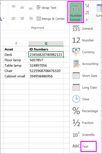
Select the cell or range of cells that contains the numbers that you want to format as text. How to select cells or a range.
Tip: You can also select empty cells, and then enter numbers after you format the cells as text. Those numbers will be formatted as text.
-
On the Home tab, in the Number group, click the arrow next to the Number Format box, and then click Text.
Note: If you don’t see the Text option, use the scroll bar to scroll to the end of the list.

Tips:
-
To use decimal places in numbers that are stored as text, you may need to include the decimal points when you type the numbers.
-
When you enter a number that begins with a zero—for example, a product code—Excel will delete the zero by default. If this is not what you want, you can create a custom number format that forces Excel to retain the leading zero. For example, if you’re typing or pasting ten-digit product codes in a worksheet, Excel will change numbers like 0784367998 to 784367998. In this case, you could create a custom number format consisting of the code 0000000000, which forces Excel to display all ten digits of the product code, including the leading zero. For more information about this issue, see Create or delete a custom number format and Keep leading zeros in number codes.
-
Occasionally, numbers might be formatted and stored in cells as text, which later can cause problems with calculations or produce confusing sort orders. This sometimes happens when you import or copy numbers from a database or other data source. In this scenario, you must convert the numbers stored as text back to numbers. For more information, see Convert numbers stored as text to numbers.
-
You can also use the TEXT function to convert a number to text in a specific number format. For examples of this technique, see Keep leading zeros in number codes. For information about using the TEXT function, see TEXT function.
Need more help?
Want more options?
Explore subscription benefits, browse training courses, learn how to secure your device, and more.
Communities help you ask and answer questions, give feedback, and hear from experts with rich knowledge.
Содержание
- Convert numbers into words
- Create the SpellNumber function to convert numbers to words
- Use the SpellNumber function in individual cells
- Save your SpellNumber function workbook
- Преобразование чисел в слова
- Создание функции SpellNumber для преобразования чисел в слова
- Использование функции SpellNumber в отдельных ячейках
- Сохранение книги с функцией SpellNumber
- Format numbers as text
- How to Convert Numbers to Text in Excel – 4 Super Easy Ways
- Why Convert Numbers to Text in Excel?
- Keeping Leading Zeros
- Entering Large Numeric Values
- Changing Numbers to Dates
- Convert Numbers to Text in Excel
- Adding an Apostrophe
- Converting Cell Format to Text
- Using the TEXT Function
- Using Text to Columns
Convert numbers into words
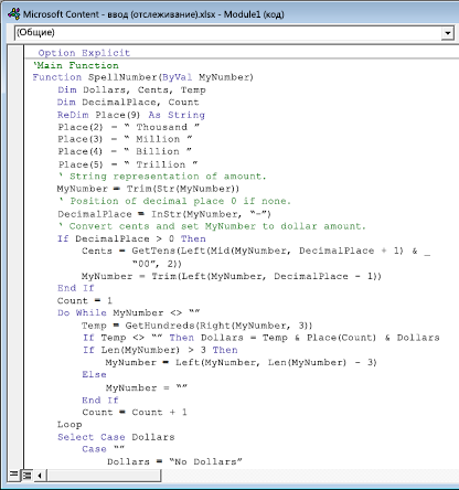
Excel doesn’t have a default function that displays numbers as English words in a worksheet, but you can add this capability by pasting the following SpellNumber function code into a VBA (Visual Basic for Applications) module. This function lets you convert dollar and cent amounts to words with a formula, so 22.50 would read as Twenty-Two Dollars and Fifty Cents. This can be very useful if you’re using Excel as a template to print checks.
If you want to convert numeric values to text format without displaying them as words, use the TEXT function instead.
Note: Microsoft provides programming examples for illustration only, without warranty either expressed or implied. This includes, but is not limited to, the implied warranties of merchantability or fitness for a particular purpose. This article assumes that you are familiar with the VBA programming language, and with the tools that are used to create and to debug procedures. Microsoft support engineers can help explain the functionality of a particular procedure. However, they will not modify these examples to provide added functionality, or construct procedures to meet your specific requirements.
Create the SpellNumber function to convert numbers to words
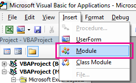
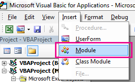
Use the keyboard shortcut, Alt + F11 to open the Visual Basic Editor (VBE).
Note: You can also access the Visual Basic Editor by showing the Developer tab in your ribbon.
Click the Insert tab, and click Module.
Copy the following lines of code.
Note: Known as a User Defined Function (UDF), this code automates the task of converting numbers to text throughout your worksheet.
Paste the lines of code into the Module1 (Code) box.
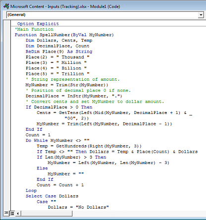
Press Alt + Q to return to Excel. The SpellNumber function is now ready to use.
Note: This function works only for the current workbook. To use this function in another workbook, you must repeat the steps to copy and paste the code in that workbook.
Use the SpellNumber function in individual cells
Type the formula =SpellNumber( A1) into the cell where you want to display a written number, where A1 is the cell containing the number you want to convert. You can also manually type the value like =SpellNumber(22.50).
Press Enter to confirm the formula.
Save your SpellNumber function workbook
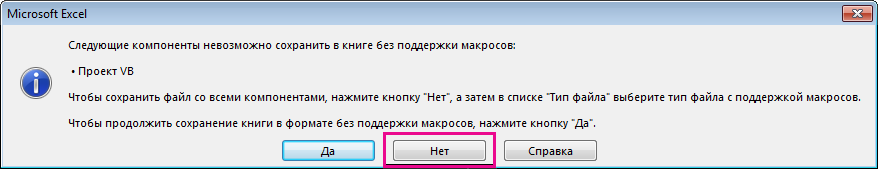
Excel cannot save a workbook with macro functions in the standard macro-free workbook format (.xlsx). If you click File > Save. A VB project dialog box opens. Click No.
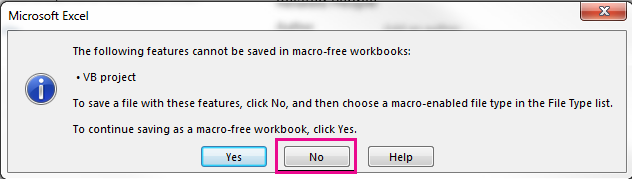
You can save your file as an Excel Macro-Enabled Workbook (.xlsm) to keep your file in its current format.
Click File > Save As.
Click the Save as type drop-down menu, and select Excel Macro-Enabled Workbook.
Источник
Преобразование чисел в слова
В Excel нет функции по умолчанию, которая отображает числа в качестве английских слов на листах, но вы можете добавить эту возможность, вклеив следующий код функции SpellNumber в модуль VBA (Visual Basic для приложений). Эта функция позволяет преобразовать суммы в рублях и центах в слова с помощью формулы, поэтому 22,50 будет читаться как Twenty-Two рублях и fifty Cents. Это может быть очень полезно, если вы используете Excel в качестве шаблона для печати проверок.
Если вы хотите преобразовать числовое значение в текстовый формат, не отображая их как слова, используйте вместо этого функцию ТЕКСТ.
Примечание: Корпорация Майкрософт предоставляет примеры программирования только для иллюстрации без каких-либо гарантий, как выраженных, так и подразумеваемых. При этом подразумеваемые гарантии пригодности для определенной цели включают, но не ограничив эту возможность. В этой статье предполагается, что вы знакомы с языком программирования VBA и средствами, которые используются для создания и отлагки процедур. Инженеры службы поддержки Майкрософт могут объяснить функциональные возможности конкретной процедуры. Однако они не будут изменять эти примеры, чтобы обеспечить дополнительные функции или создавать процедуры в порядке, отвечая вашим требованиям.
Создание функции SpellNumber для преобразования чисел в слова
Используйте клавиши ALT+F11, чтобы открыть редактор Visual Basic (VBE).
Примечание: Вы также можете открывать редактор Visual Basic, добавив вкладку «Разработчик» на ленту.
На вкладке Insert (Вставка) нажмите кнопку Module (Модуль).
Скопируйте приведенный ниже код.
Примечание: Этот код автоматизирует преобразование чисел в текст на всем компьютере.
Вставьте строки кода в поле Module1 (Code) (Модуль 1 — код).
Нажмите ALT+Q, чтобы вернуться в Excel. Функция SpellNumber готова к использованию.
Примечание: Эта функция работает только для текущей книги. Чтобы использовать эту функцию в другой книге, необходимо повторить действия по копированию и вкопии кода в нее.
Использование функции SpellNumber в отдельных ячейках
Введите формулу =SpellNumber (A1)в ячейку, в которой нужно отобразить записанное число, где A1 — это ячейка с числом, преобразуемом в ячейку. Вы также можете ввести значение вручную, например =SpellNumber(22,50).
Нажмите ввод, чтобы подтвердить формулу.
Сохранение книги с функцией SpellNumber
В Excel не удается сохранить книгу с функциями макроса в стандартном формате книги без макроса (XLSX). Если нажать кнопку «> сохранить». Откроется диалоговое окно проекта VB. щелкните Нет.
Вы можете сохранить файл как книгу Excel Macro-Enabled (XLSM), чтобы сохранить его в текущем формате.
На вкладке Файл выберите команду Сохранить как.
В меню «Тип сохранения» выберите пункт «Macro-Enabled Excel».
Источник
Format numbers as text
If you want Excel to treat certain types of numbers as text, you can use the text format instead of a number format. For example, If you are using credit card numbers, or other number codes that contain 16 digits or more, you must use a text format. That’s because Excel has a maximum of 15 digits of precision and will round any numbers that follow the 15th digit down to zero, which probably isn’t what you want to happen.
It’s easy to tell at a glance if a number is formatted as text, because it will be left-aligned instead of right-aligned in the cell.
Select the cell or range of cells that contains the numbers that you want to format as text. How to select cells or a range.
Tip: You can also select empty cells, and then enter numbers after you format the cells as text. Those numbers will be formatted as text.
On the Home tab, in the Number group, click the arrow next to the Number Format box, and then click Text.
Note: If you don’t see the Text option, use the scroll bar to scroll to the end of the list.
To use decimal places in numbers that are stored as text, you may need to include the decimal points when you type the numbers.
When you enter a number that begins with a zero—for example, a product code—Excel will delete the zero by default. If this is not what you want, you can create a custom number format that forces Excel to retain the leading zero. For example, if you’re typing or pasting ten-digit product codes in a worksheet, Excel will change numbers like 0784367998 to 784367998. In this case, you could create a custom number format consisting of the code 0000000000, which forces Excel to display all ten digits of the product code, including the leading zero. For more information about this issue, see Create or delete a custom number format and Keep leading zeros in number codes.
Occasionally, numbers might be formatted and stored in cells as text, which later can cause problems with calculations or produce confusing sort orders. This sometimes happens when you import or copy numbers from a database or other data source. In this scenario, you must convert the numbers stored as text back to numbers. For more information, see Convert numbers stored as text to numbers.
You can also use the TEXT function to convert a number to text in a specific number format. For examples of this technique, see Keep leading zeros in number codes. For information about using the TEXT function, see TEXT function.
Источник
How to Convert Numbers to Text in Excel – 4 Super Easy Ways
Excel is a great tool which can be used for data entry, as a database, and to analyze data and create dashboards and reports.
While most of the in-built features and default settings are meant to be useful and save time for the users, sometimes, you may want to change things a little.
Converting your numbers into text is one such scenario.
In this tutorial, I will show you some easy ways to quickly convert numbers to text in Excel.
This Tutorial Covers:
Why Convert Numbers to Text in Excel?
When working with numbers in Excel, it’s best to keep these as numbers only. But in some cases, having a number could actually be a problem.
Lets look at a couple of scenarios where having numbers creates issues for the users.
Keeping Leading Zeros
For example, if you enter 001 in a cell in Excel, you will notice that Excel automatically removes the leading zeros (as it thinks these are unnecessary).
While this is not an issue in most cases (as you wouldn’t leading zeros), in case you do need these then one of the solutions is to convert these numbers to text.
This way, you get exactly what you enter.
One common scenario where you might need this is when you’re working with large numbers – such as SSN or employee ids that have leading zeros.
Entering Large Numeric Values
Do you know that you can only enter a numeric value that is 15 digits long in Excel? If you enter a 16 digit long number, it will change the 16th digit to 0.
So if you are working with SSN, account numbers, or any other type of large numbers, there is a possibility that your input data is automatically being changed by Excel.
And what’s even worse is that you don’t get any prompt or error. It just changes the digits to 0 after the 15th digit.
Again, this is something that is taken care of if you convert the number to text.
Changing Numbers to Dates
This one erk a lot of people (including myself).
Try entering 01-01 in Excel and it will automatically change it to date (01 January of the current year).
So if you enter anything that is a valid date format in Excel, it would be converted to a date.
A lot of people reach out to me for this as they want to enter scores in Excel in this format, but end up getting frustrated when they see dates instead.
Again, changing the format of the cell from number to text will help keep the scores as is.
Now, let’s go ahead and have a look at some of the methods you can use to convert numbers to text in Excel.
Convert Numbers to Text in Excel
In this section, I will cover four different ways you can use to convert numbers to text in Excel.
Not all these methods are the same and some would be more suitable than others depending on your situation.
So let’s dive in!
Adding an Apostrophe
If you manually entering data in Excel and you don’t want your numbers to change the format automatically, here is a simple trick:
Add an apostrophe (‘) before the number
So if you want to enter 001, enter ‘001 (where there is an apostrophe before the number).
And don’t worry, the apostrophe is not visible in the cell. You will only see the number.
When you add an apostrophe before a number, it will change it to text and also add a small green triangle at the top left part of the cell (as shown in th image). It’s Exel way to letting you know that the cell has a number that has been converted to text.
When you add an apostrophe before a number, it tells Excel to consider whatever follows as text.
A quick way to visually confirm whether the cells are formatted as text or not is to see whether the numbers align to the left out to the right. When numbers are formatted as text, they align to the right by default (as they alight to the left)
Even if you add an apostrophe before a number in a cell in Excel, you can still use these as numbers in calculations
Similarly, if you want to enter 01-01, adding an apostrophe would make sure that it doesn’t get changed into a date.
Although this technique works in all cases, it is only useful if you’re manually entering a few numbers in Excel. If you enter a lot of data in a specific range of rows/columns, use the next method.
Converting Cell Format to Text
Another way to make sure that any numeric entry in Excel is considered a text value is by changing the format of the cell.
This way, you don’t have to worry about entering an apostrophe every time you manually enter the data.
You can go ahead entering the data just like you usually do, and Excel would make sure that your numbers are not changed.
Here is how to do this:
- Select the range or rows/column where you would be entering the data
- Click the Home tab
- In the Number group, click on the format drop down
- Select Text from the options that show up
The above steps would change the default formatting of the cells from General to Text.
Now, if you enter any number or any text string in these cells, it would automatically be considered as a text string.
This means that Excel would not automatically change the text you enter (such as truncating the leading zeros or converting entered numbers into dates)
In this example, while I changed the cell formatting first before entering the data, you can also do this with cells that already have data in them.
But remember that if you already had entered numbers that were changed by Excel (such as removing leading zeros or changing text to dates), that won’t come back. You will have to make that data entry again.
Also, keep in mind that cell formatting can change in case you copy and paste some data to these cells. With regular copy-paste, it also copied the formatting from the copied cells. So it’s best to copy and paste values only.
Using the TEXT Function
Excel has an in-built TEXT function that is meant to convert a numeric value to a text value (where you have to specify the format of the text in which you want to get the final result).
This method is useful when you already have a set of numbers and you want to show them in a more readable format or if you want to add some text as suffix or prefix to these numbers.
Suppose you have a set of numbers as shown below, and you want to show all these numbers as five-digit values (which means to add leading zeros to numbers that are less than 5 digits).
While Excel removes any leading zeros in numbers, you can use the below formula to get this:
In the above formula, I have used “00000” as the second argument, which tells the formula the format of the output I desire. In this example, 00000 would mean that I need all the numbers to be at least five-digit long.
You can do a lot more with the TEXT function – such as add currency symbol, add prefix or suffix to the numbers, or change the format to have comma or decimals.
Using this method can be useful when you already have the data in Excel and you want to format it in a specific way.
This can also be helpful in saving time when doing manual data entry, where you can quickly enter the data and then use the TEXT function to get it in the desired format.
Using Text to Columns
Another quick way to convert numbers to text in Excel is by using the Text to Columns wizard.
While the purpose of Text to Columns is to split the data into multiple columns, it has a setting that also allows us to quickly select a range of cells and convert all the numbers into text with a few clicks.
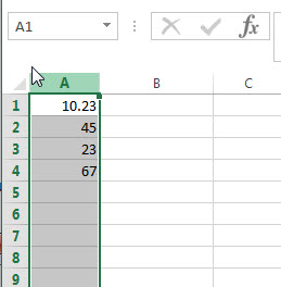
Suppose you have a data set is shown below, and you want to convert all the numbers in columns A into text.
Below are the steps to do this:
- Select the numbers in Column A
- Click the Data tab
- Click on the Text to Columns icon in the ribbon. This will open the text to columns wizard this will open the text to column wizard
- In Step 1 of 3, click the Next button
- In Step 2 of 3, click the Next button
- In Step 3 of 3, under the ‘Column data format’ options, select Text
The above steps would instantly convert all these numbers in Column A into text. You notice that the numbers would now be aligned to the right (indicating that the cell content is text).
There would also be a small green triangle at the top left part of the cell, which is a way Excel informs you that there are numbers that are stored as text.
So these are four easy ways that you can use to quickly convert numbers to text in Excel.
In case you only want this for a few cells where you would be manually entering the data, I suggest you use the apostrophe method. If you need to do data entry for more than a few cells, you can try changing the format of the cells from General to Text.
And in case you already have the numbers in Excel and you want to convert them to text, you can use the TEXT formula method or the Text to Columns method I covered in this tutorial.
I hope you found this tutorial useful.
Other Excel tutorials you may also like:
Источник
Содержание
- Конвертация числа в текстовый вид
- Способ 1: форматирование через контекстное меню
- Способ 2: инструменты на ленте
- Способ 3: использование функции
- Конвертация текста в число
- Способ 1: преобразование с помощью значка об ошибке
- Способ 2: конвертация при помощи окна форматирования
- Способ 3: конвертация посредством инструментов на ленте
- Способ 4: применение формулы
- Способ 5: применение специальной вставки
- Способ 6: использование инструмента «Текст столбцами»
- Способ 7: применение макросов
- Вопросы и ответы

Одной из частых задач, с которыми сталкиваются пользователи программы Эксель, является преобразования числовых выражений в текстовый формат и обратно. Этот вопрос часто заставляет потратить на решение много времени, если юзер не знает четкого алгоритма действий. Давайте разберемся, как можно решить обе задачи различными способами.
Конвертация числа в текстовый вид
Все ячейки в Экселе имеют определенный формат, который задает программе, как ей рассматривать то или иное выражение. Например, даже если в них будут записаны цифры, но формат выставлен текстовый, то приложение будет рассматривать их, как простой текст, и не сможет проводить с такими данными математические вычисления. Для того, чтобы Excel воспринимал цифры именно как число, они должны быть вписаны в элемент листа с общим или числовым форматом.
Для начала рассмотрим различные варианты решения задачи конвертации чисел в текстовый вид.
Способ 1: форматирование через контекстное меню
Чаще всего пользователи выполняют форматирование числовых выражений в текстовые через контекстное меню.
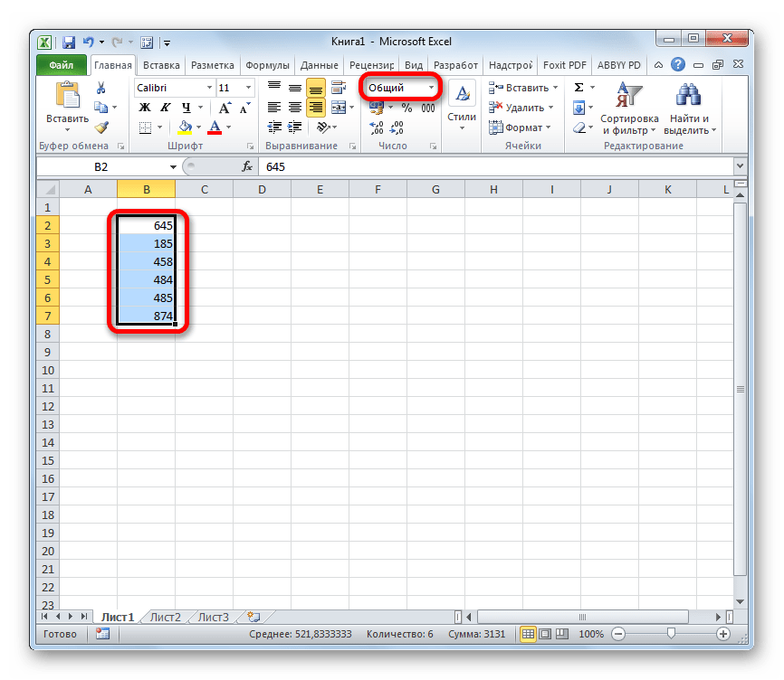
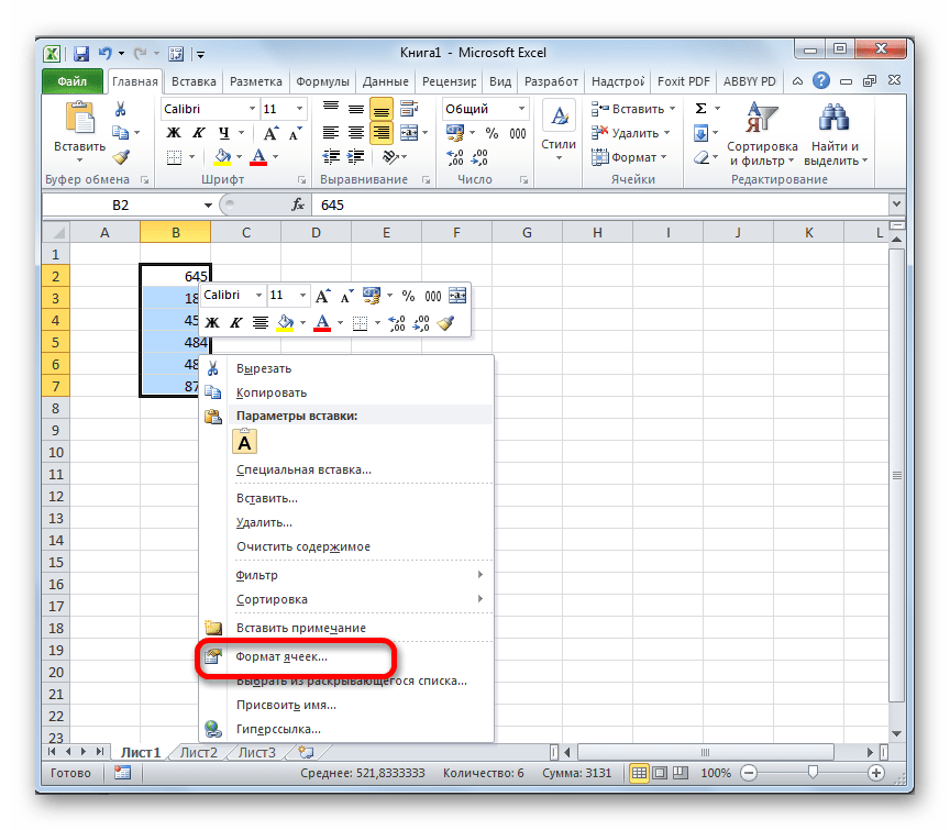
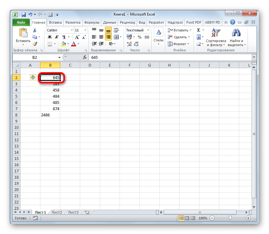
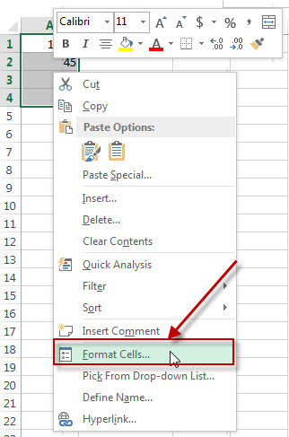
- Выделяем те элементы листа, в которых нужно преобразовать данные в текст. Как видим, во вкладке «Главная» на панели инструментов в блоке «Число» в специальном поле отображается информация о том, что данные элементы имеют общий формат, а значит, цифры, вписанные в них, воспринимаются программой, как число.
- Кликаем правой кнопкой мыши по выделению и в открывшемся меню выбираем позицию «Формат ячеек…».
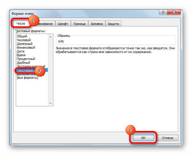
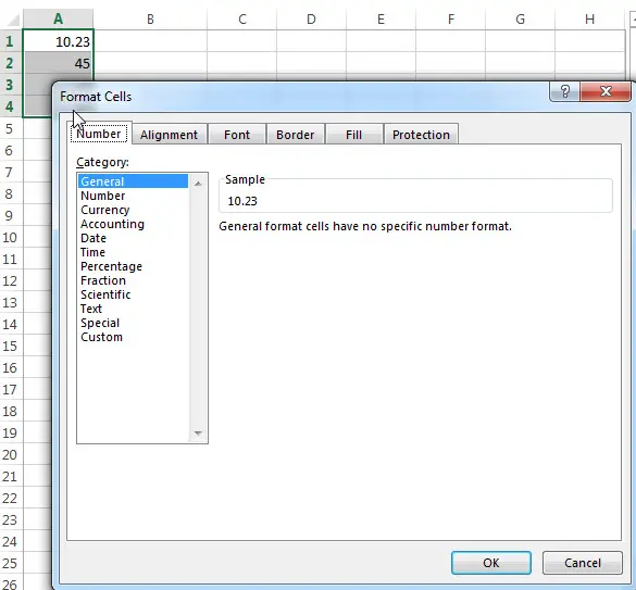
- В открывшемся окне форматирования переходим во вкладку «Число», если оно было открыто в другом месте. В блоке настроек «Числовые форматы» выбираем позицию «Текстовый». Для сохранения изменений жмем на кнопку «OK» в нижней части окна.
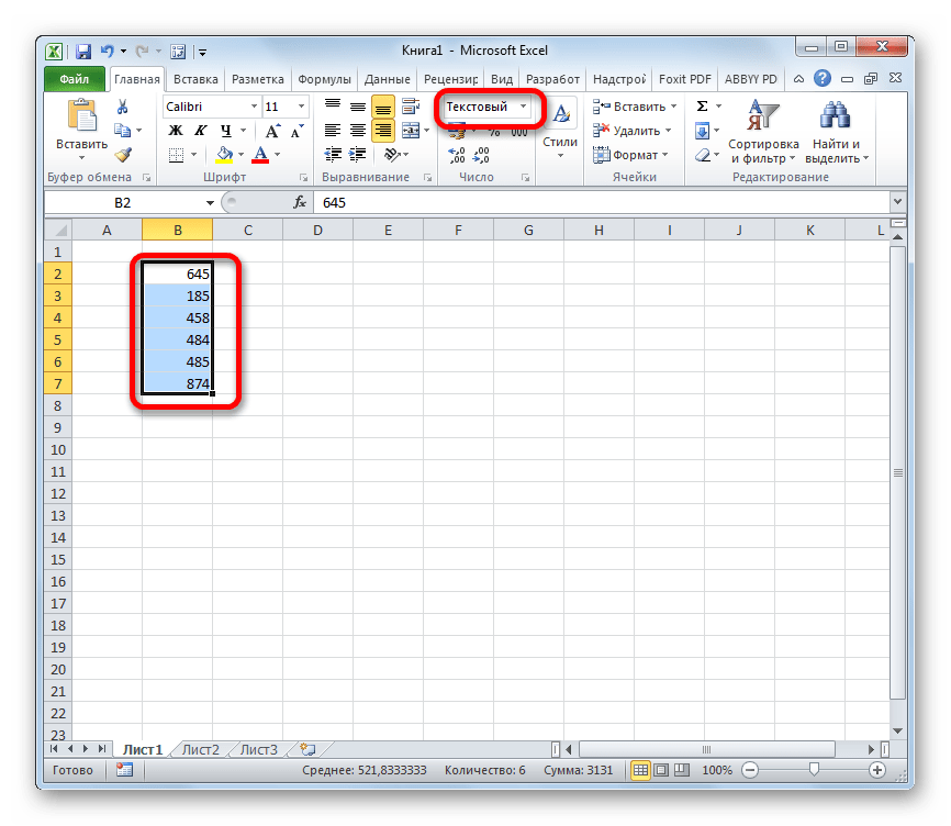
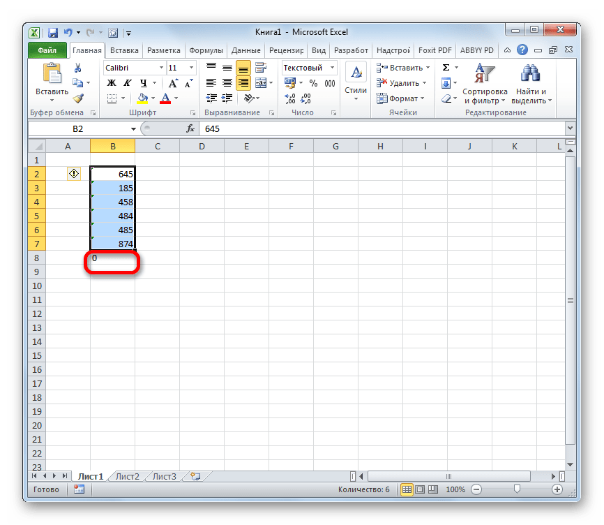
- Как видим, после данных манипуляций в специальном поле высвечивается информация о том, что ячейки были преобразованы в текстовый вид.
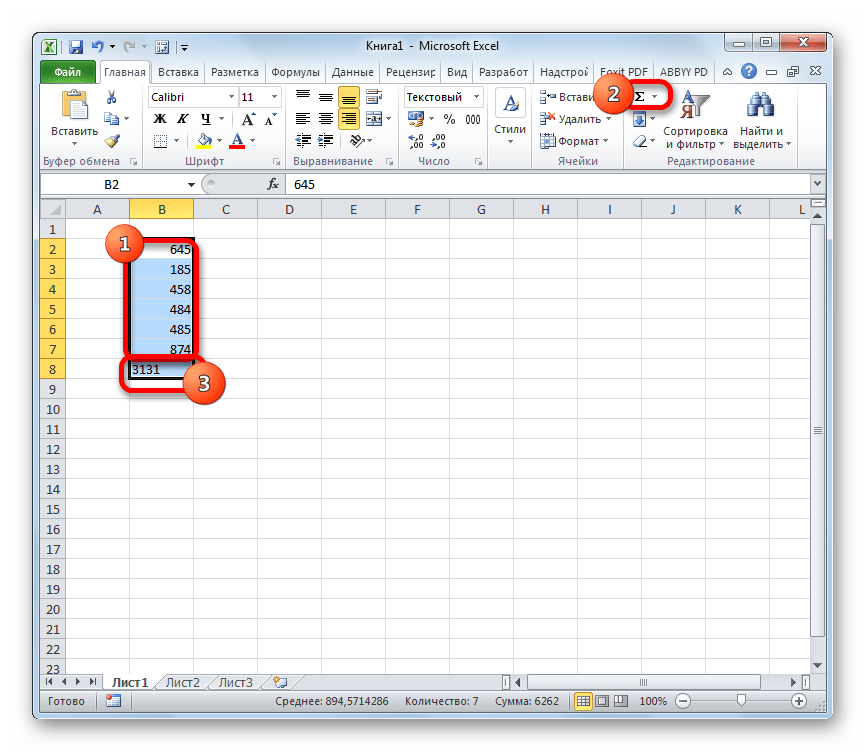
- Но если мы попытаемся подсчитать автосумму, то она отобразится в ячейке ниже. Это означает, что преобразование было совершено не полностью. В этом и заключается одна из фишек Excel. Программа не дает завершить преобразование данных наиболее интуитивно понятным способом.
- Чтобы завершить преобразование, нам нужно последовательно двойным щелчком левой кнопки мыши поместить курсор в каждый элемент диапазона в отдельности и нажать на клавишу Enter. Чтобы упростить задачу вместо двойного щелчка можно использовать нажатие функциональной клавиши F2.
- После выполнения данной процедуры со всеми ячейками области, данные в них будут восприниматься программой, как текстовые выражения, а, следовательно, и автосумма будет равна нулю. Кроме того, как видим, левый верхний угол ячеек будет окрашен в зеленый цвет. Это также является косвенным признаком того, что элементы, в которых находятся цифры, преобразованы в текстовый вариант отображения. Хотя этот признак не всегда является обязательным и в некоторых случаях такая пометка отсутствует.
Урок: Как изменить формат в Excel
Способ 2: инструменты на ленте
Преобразовать число в текстовый вид можно также воспользовавшись инструментами на ленте, в частности, использовав поле для показа формата, о котором шел разговор выше.
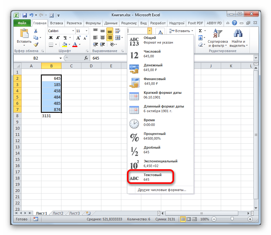
- Выделяем элементы, данные в которых нужно преобразовать в текстовый вид. Находясь во вкладке «Главная» кликаем по пиктограмме в виде треугольника справа от поля, в котором отображается формат. Оно расположено в блоке инструментов «Число».
- В открывшемся перечне вариантов форматирования выбираем пункт «Текстовый».
- Далее, как и в предыдущем способе, последовательно устанавливаем курсор в каждый элемент диапазона двойным щелчком левой кнопки мыши или нажатием клавиши F2, а затем щелкаем по клавише Enter.
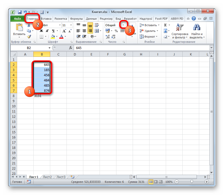

Данные преобразовываются в текстовый вариант.
Способ 3: использование функции
Ещё одним вариантом преобразования числовых данных в тестовые в Экселе является применение специальной функции, которая так и называется – ТЕКСТ. Данный способ подойдёт, в первую очередь, если вы хотите перенести числа как текст в отдельный столбец. Кроме того, он позволит сэкономить время на преобразовании, если объем данных слишком большой. Ведь, согласитесь, что перещелкивать каждую ячейку в диапазоне, насчитывающем сотни или тысячи строк – это не самый лучший выход.
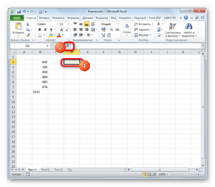
- Устанавливаем курсор в первый элемент диапазона, в котором будет выводиться результат преобразования. Щелкаем по значку «Вставить функцию», который размещен около строки формул.
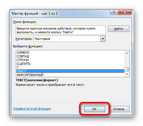
- Запускается окно Мастера функций. В категории «Текстовые» выделяем пункт «ТЕКСТ». После этого кликаем по кнопке «OK».
- Открывается окно аргументов оператора ТЕКСТ. Данная функция имеет следующий синтаксис:
=ТЕКСТ(значение;формат)Открывшееся окно имеет два поля, которые соответствуют данным аргументам: «Значение» и «Формат».
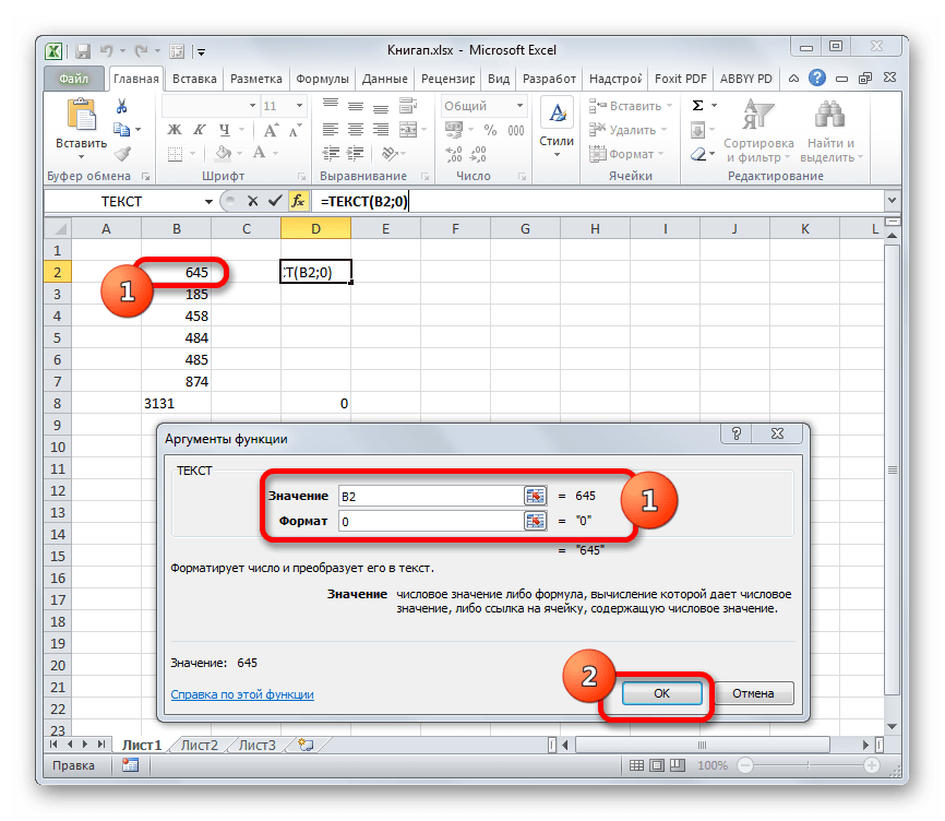
В поле «Значение» нужно указать преобразовываемое число или ссылку на ячейку, в которой оно находится. В нашем случае это будет ссылка на первый элемент обрабатываемого числового диапазона.
В поле «Формат» нужно указать вариант отображения результата. Например, если мы введем «0», то текстовый вариант на выходе будет отображаться без десятичных знаков, даже если в исходнике они были. Если мы внесем «0,0», то результат будет отображаться с одним десятичным знаком, если «0,00», то с двумя, и т.д.
После того, как все требуемые параметры введены, щелкаем по кнопке «OK».
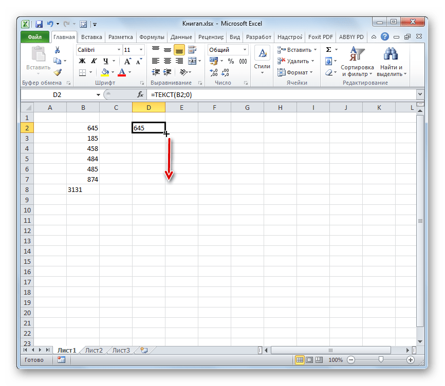
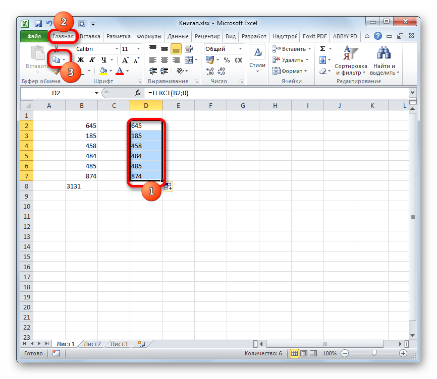
- Как видим, значение первого элемента заданного диапазона отобразилось в ячейке, которую мы выделили ещё в первом пункте данного руководства. Для того, чтобы перенести и другие значения, нужно скопировать формулу в смежные элементы листа. Устанавливаем курсор в нижний правый угол элемента, который содержит формулу. Курсор преобразуется в маркер заполнения, имеющий вид небольшого крестика. Зажимаем левую кнопку мыши и протаскиваем по пустым ячейкам параллельно диапазону, в котором находятся исходные данные.
- Теперь весь ряд заполнен требуемыми данными. Но и это ещё не все. По сути, все элементы нового диапазона содержат в себе формулы. Выделяем эту область и жмем на значок «Копировать», который расположен во вкладке «Главная» на ленте инструментов группе «Буфер обмена».
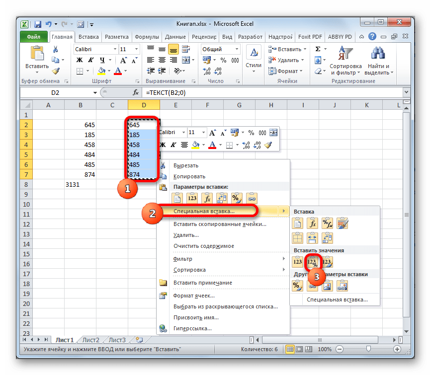
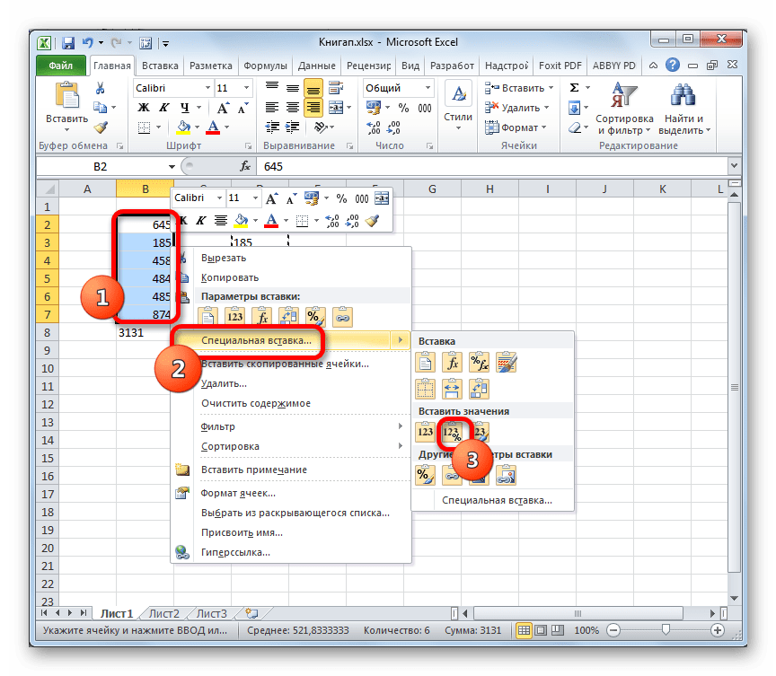
- Далее, если мы хотим сохранить оба диапазона (исходный и преобразованный), не снимаем выделение с области, которая содержит формулы. Кликаем по ней правой кнопкой мыши. Происходит запуск контекстного списка действий. Выбираем в нем позицию «Специальная вставка». Среди вариантов действий в открывшемся списке выбираем «Значения и форматы чисел».

Если же пользователь желает заменить данные исходного формата, то вместо указанного действия нужно выделить именно его и произвести вставку тем же способом, который указан выше.
- В любом случае, в выбранный диапазон будут вставлены данные в текстовом виде. Если же вы все-таки выбрали вставку в исходную область, то ячейки, содержащие формулы, можно очистить. Для этого выделяем их, кликаем правой кнопкой мыши и выбираем позицию «Очистить содержимое».
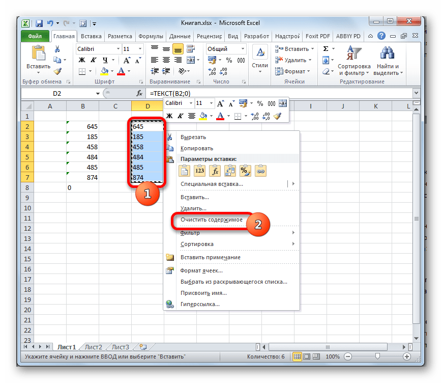
На этом процедуру преобразования можно считать оконченной.
Урок: Мастер функций в Excel
Конвертация текста в число
Теперь давайте разберемся, какими способами можно выполнить обратную задачу, а именно как преобразовать текст в число в Excel.
Способ 1: преобразование с помощью значка об ошибке
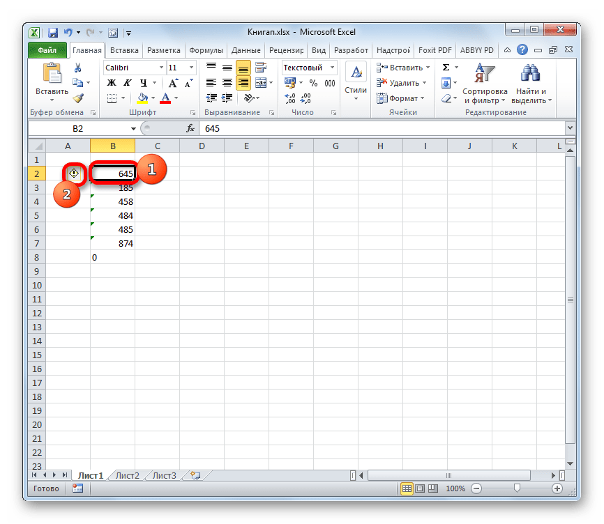
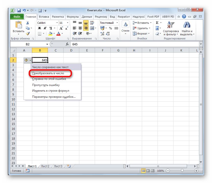
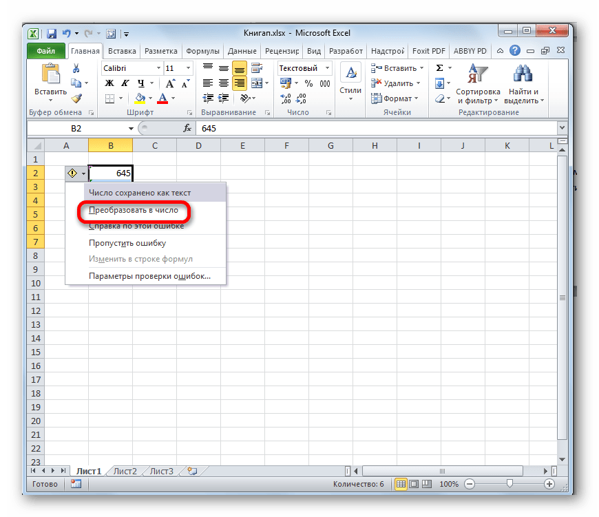
Проще и быстрее всего выполнить конвертацию текстового варианта с помощью специального значка, который сообщает об ошибке. Этот значок имеет вид восклицательного знака, вписанного в пиктограмму в виде ромба. Он появляется при выделении ячеек, которые имеют пометку в левом верхнем углу зеленым цветом, обсуждаемую нами ранее. Эта пометка ещё не свидетельствует о том, что данные находящиеся в ячейке обязательно ошибочные. Но цифры, расположенные в ячейке имеющей текстовый вид, вызывают подозрения у программы в том, что данные могут быть внесены некорректно. Поэтому на всякий случай она их помечает, чтобы пользователь обратил внимание. Но, к сожалению, такие пометки Эксель выдает не всегда даже тогда, когда цифры представлены в текстовом виде, поэтому ниже описанный способ подходит не для всех случаев.
- Выделяем ячейку, в которой содержится зеленый индикатор о возможной ошибке. Кликаем по появившейся пиктограмме.
- Открывается список действий. Выбираем в нем значение «Преобразовать в число».
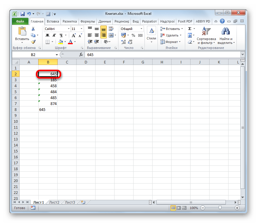
- В выделенном элементе данные тут же будут преобразованы в числовой вид.
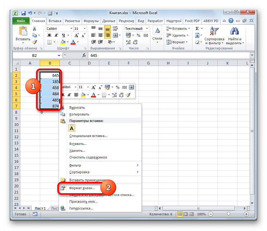
Если подобных текстовых значений, которые следует преобразовать, не одно, а множество, то в этом случае можно ускорить процедуру преобразования.
- Выделяем весь диапазон, в котором находятся текстовые данные. Как видим, пиктограмма появилась одна для всей области, а не для каждой ячейки в отдельности. Щелкаем по ней.
- Открывается уже знакомый нам список. Как и в прошлый раз, выбираем позицию «Преобразовать в число».
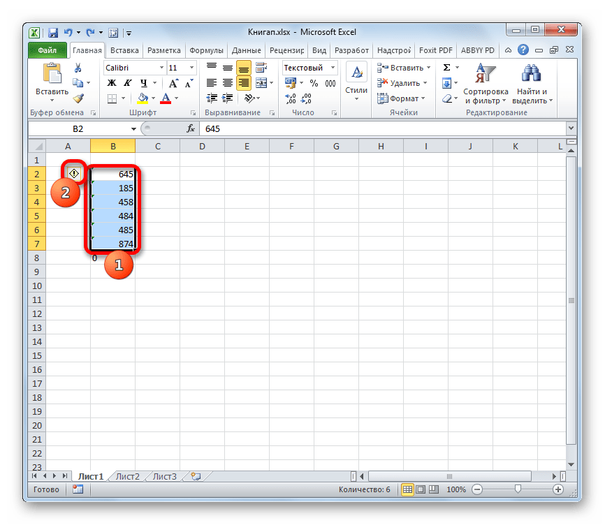
Все данные массива будут преобразованы в указанный вид.

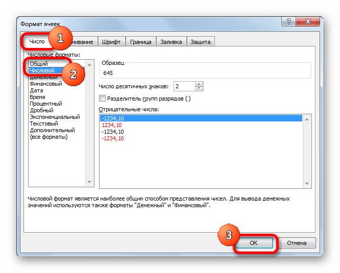
Способ 2: конвертация при помощи окна форматирования
Как и для преобразования данных из числового вида в текст, в Экселе существует возможность обратного конвертирования через окно форматирования.
- Выделяем диапазон, содержащий цифры в текстовом варианте. Кликаем правой кнопкой мыши. В контекстном меню выбираем позицию «Формат ячеек…».
- Выполняется запуск окна форматирования. Как и в предыдущий раз, переходим во вкладку «Число». В группе «Числовые форматы» нам нужно выбрать значения, которые позволят преобразовать текст в число. К ним относится пункты «Общий» и «Числовой». Какой бы из них вы не выбрали, программа будет расценивать цифры, введенные в ячейку, как числа. Производим выбор и жмем на кнопку. Если вы выбрали значение «Числовой», то в правой части окна появится возможность отрегулировать представление числа: выставить количество десятичных знаков после запятой, установить разделителями между разрядами. После того, как настройка выполнена, жмем на кнопку «OK».
- Теперь, как и в случае преобразования числа в текст, нам нужно прощелкать все ячейки, установив в каждую из них курсор и нажав после этого клавишу Enter.

После выполнения этих действий все значения выбранного диапазона преобразуются в нужный нам вид.
Способ 3: конвертация посредством инструментов на ленте
Перевести текстовые данные в числовые можно, воспользовавшись специальным полем на ленте инструментов.
- Выделяем диапазон, который должен подвергнуться трансформации. Переходим во вкладку «Главная» на ленте. Кликаем по полю с выбором формата в группе «Число». Выбираем пункт «Числовой» или «Общий».
- Далее прощелкиваем уже не раз описанным нами способом каждую ячейку преобразуемой области с применением клавиш F2 и Enter.
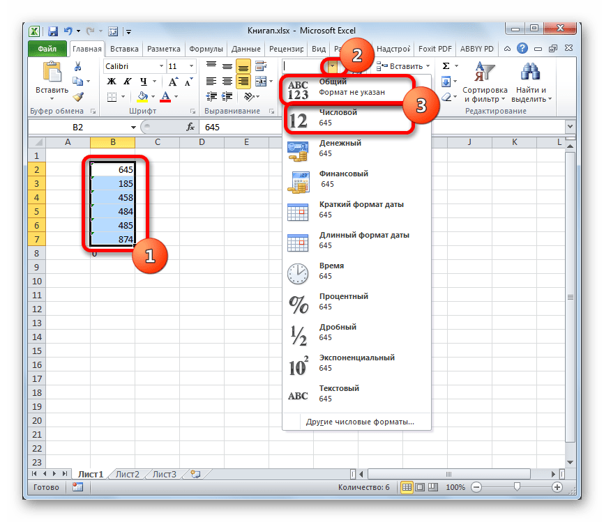
Значения в диапазоне будут преобразованы из текстовых в числовые.
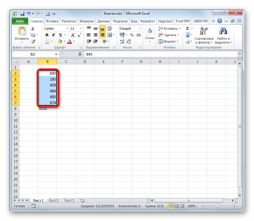
Способ 4: применение формулы
Также для преобразования текстовых значений в числовые можно использовать специальные формулы. Рассмотрим, как это сделать на практике.
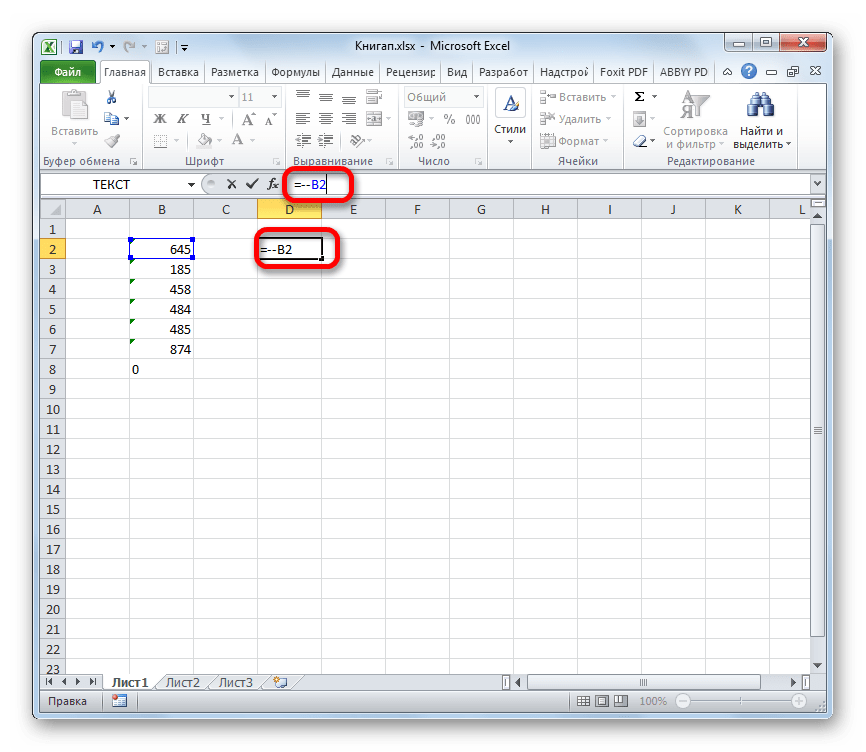
- В пустой ячейке, расположенной параллельно первому элементу диапазона, который следует преобразовать, ставим знак «равно» (=) и двойной символ «минус» (—). Далее указываем адрес первого элемента трансформируемого диапазона. Таким образом, происходит двойное умножение на значение «-1». Как известно, умножение «минус» на «минус» дает «плюс». То есть, в целевой ячейке мы получаем то же значение, которое было изначально, но уже в числовом виде. Даная процедура называется двойным бинарным отрицанием.
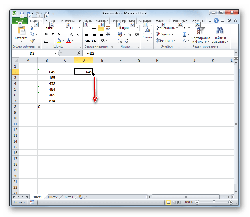
- Жмем на клавишу Enter, после чего получаем готовое преобразованное значение. Для того, чтобы применить данную формулу для всех других ячеек диапазона, используем маркер заполнения, который ранее был применен нами для функции ТЕКСТ.
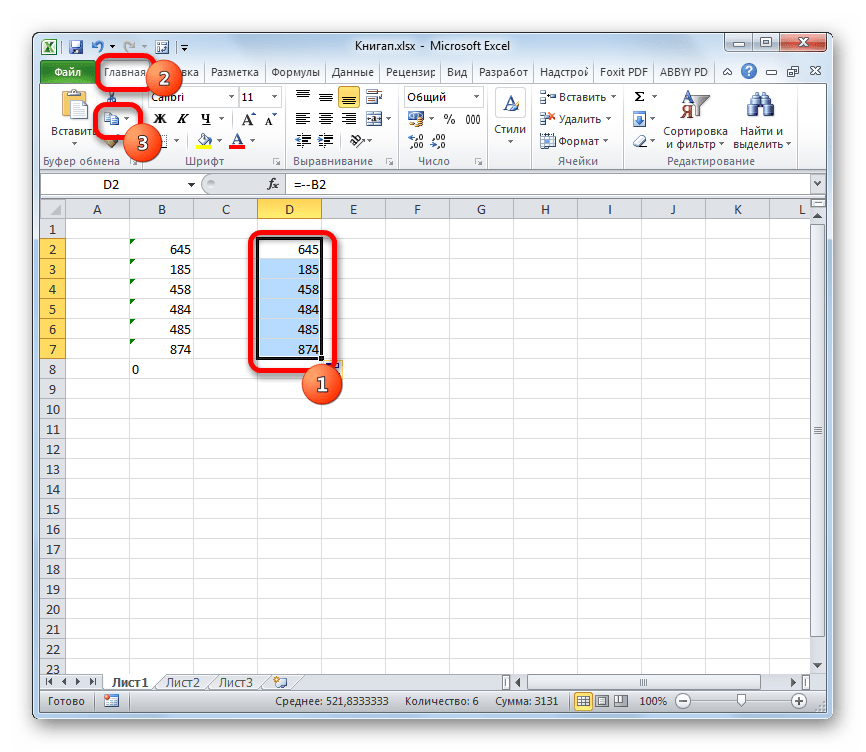
- Теперь мы имеем диапазон, который заполнен значениями с формулами. Выделяем его и жмем на кнопку «Копировать» во вкладке «Главная» или применяем сочетание клавиш Ctrl+C.
- Выделяем исходную область и производим щелчок по ней правой кнопкой мыши. В активировавшемся контекстном списке переходим по пунктам «Специальная вставка» и «Значения и форматы чисел».
- Все данные вставлены в нужном нам виде. Теперь можно удалить транзитный диапазон, в котором находится формула двойного бинарного отрицания. Для этого выделяем данную область, кликом правой кнопки мыши вызываем контекстное меню и выбираем в нем позицию «Очистить содержимое».
Кстати, для преобразования значений данным методом совсем не обязательно использовать исключительно двойное умножение на «-1». Можно применять любое другое арифметическое действие, которое не ведет к изменению значений (сложение или вычитание нуля, выполнение возведения в первую степень и т.д.)
Урок: Как сделать автозаполнение в Excel
Способ 5: применение специальной вставки
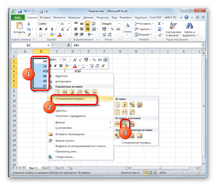
Следующий способ по принципу действия очень похож на предыдущий с той лишь разницей, что для его использования не нужно создавать дополнительный столбец.
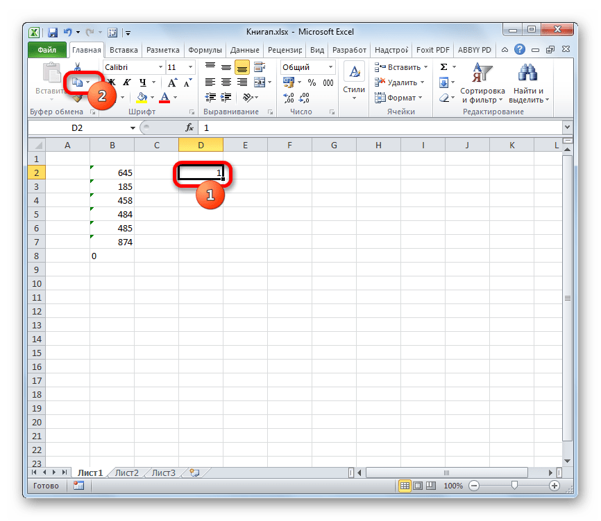
- В любую пустую ячейку на листе вписываем цифру «1». Затем выделяем её и жмем на знакомый значок «Копировать» на ленте.
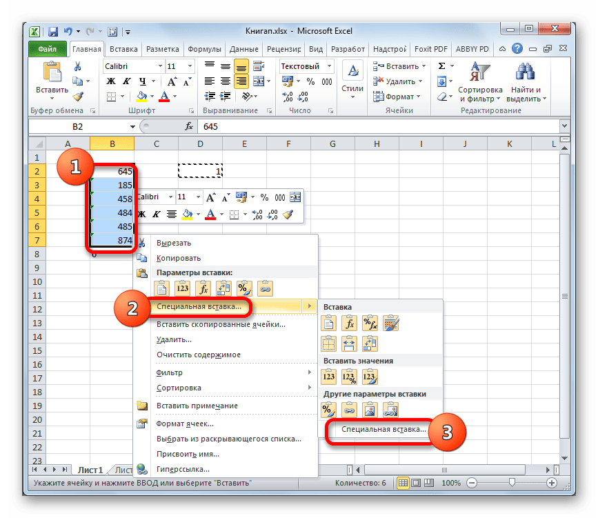
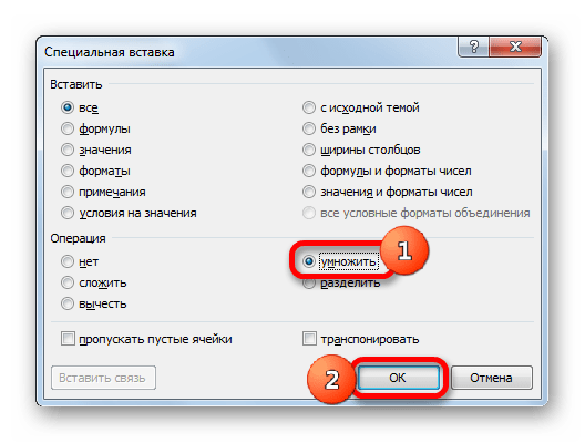
- Выделяем область на листе, которую следует преобразовать. Кликаем по ней правой кнопкой мыши. В открывшемся меню дважды переходим по пункту «Специальная вставка».
- В окне специальной вставки выставляем переключатель в блоке «Операция» в позицию «Умножить». Вслед за этим жмем на кнопку «OK».
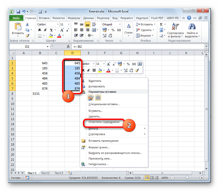
- После этого действия все значения выделенной области будут преобразованы в числовые. Теперь при желании можно удалить цифру «1», которую мы использовали в целях конвертации.

Способ 6: использование инструмента «Текст столбцами»
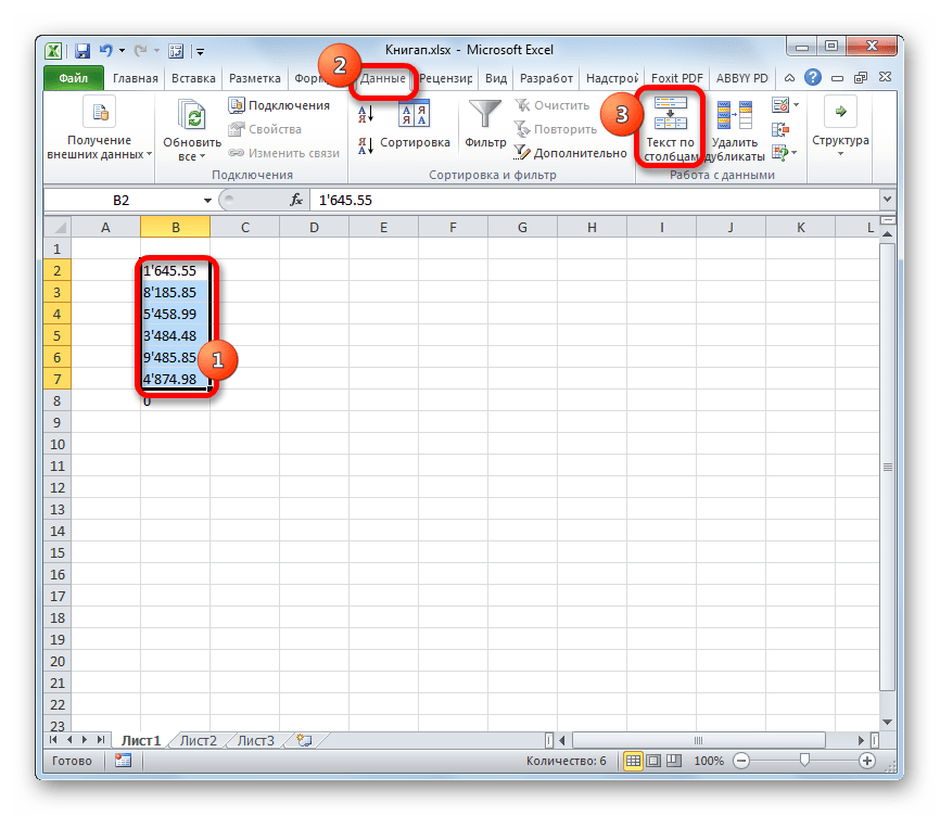
Ещё одним вариантом, при котором можно преобразовать текст в числовой вид, является применение инструмента «Текст столбцами». Его есть смысл использовать тогда, когда вместо запятой в качестве разделителя десятичных знаков используется точка, а в качестве разделителя разрядов вместо пробела – апостроф. Этот вариант воспринимается в англоязычном Экселе, как числовой, но в русскоязычной версии этой программы все значения, которые содержат указанные выше знаки, воспринимаются как текст. Конечно, можно перебить данные вручную, но если их много, это займет значительное количество времени, тем более что существует возможность гораздо более быстрого решения проблемы.
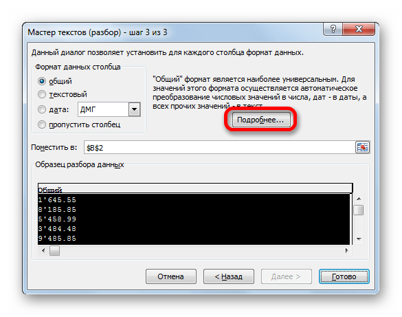
- Выделяем фрагмент листа, содержимое которого нужно преобразовать. Переходим во вкладку «Данные». На ленте инструментов в блоке «Работа с данными» кликаем по значку «Текст по столбцам».
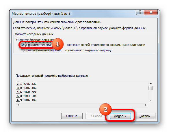
- Запускается Мастер текстов. В первом окне обратите внимание, чтобы переключатель формата данных стоял в позиции «С разделителями». По умолчанию он должен находиться в этой позиции, но проверить состояние будет не лишним. Затем кликаем по кнопке «Далее».
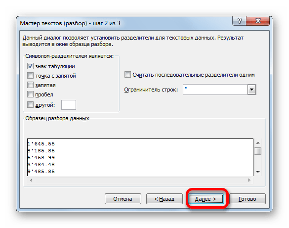
- Во втором окне также оставляем все без изменений и жмем на кнопку «Далее».
- А вот после открытия третьего окна Мастера текстов нужно нажать на кнопку «Подробнее».
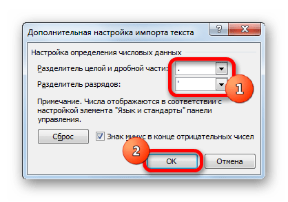
- Открывается окно дополнительной настройки импорта текста. В поле «Разделитель целой и дробной части» устанавливаем точку, а в поле «Разделитель разрядов» — апостроф. Затем делаем один щелчок по кнопке «OK».
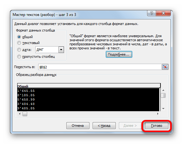
- Возвращаемся в третье окно Мастера текстов и жмем на кнопку «Готово».
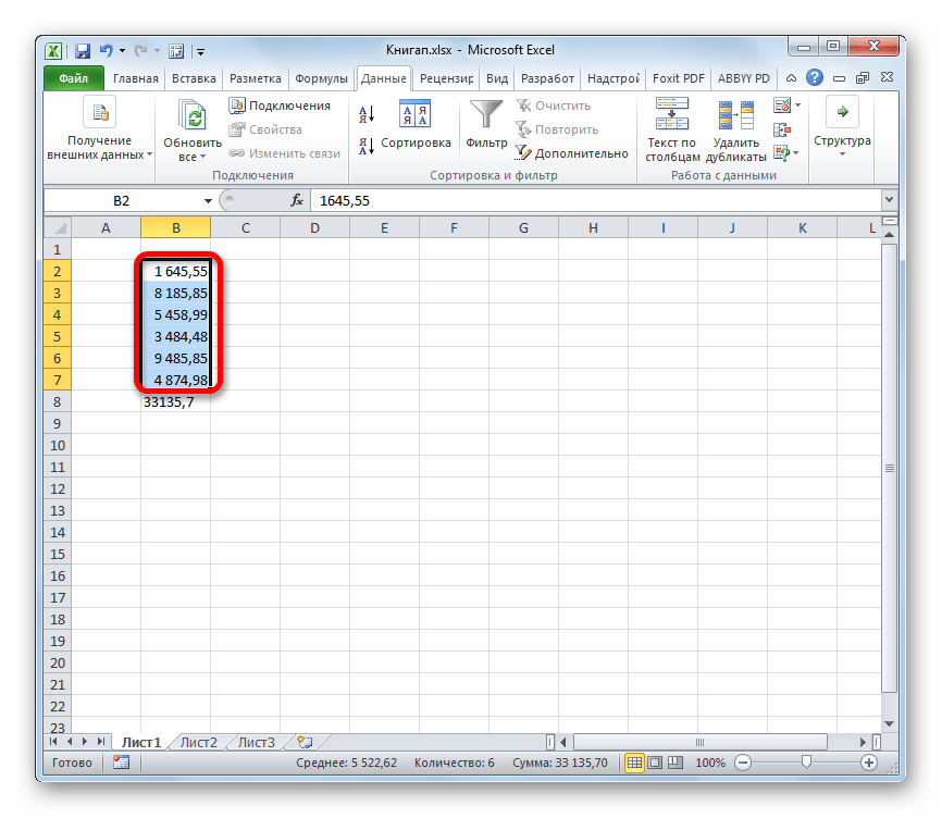
- Как видим, после выполнения данных действий числа приняли привычный для русскоязычной версии формат, а это значит, что они одновременно были преобразованы из текстовых данных в числовые.
Способ 7: применение макросов
Если вам часто приходится преобразовывать большие области данных из текстового формата в числовой, то имеется смысл в этих целях записать специальный макрос, который будет использоваться при необходимости. Но для того, чтобы это выполнить, прежде всего, нужно в своей версии Экселя включить макросы и панель разработчика, если это до сих пор не сделано.
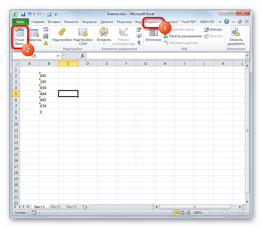
- Переходим во вкладку «Разработчик». Жмем на значок на ленте «Visual Basic», который размещен в группе «Код».
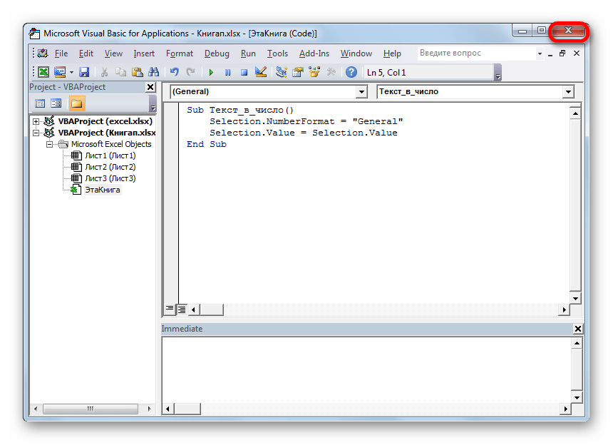
- Запускается стандартный редактор макросов. Вбиваем или копируем в него следующее выражение:
Sub Текст_в_число()

 Selection.NumberFormat = "General"

 Selection.Value = Selection.Value

End Sub
После этого закрываем редактор, выполнив нажатие стандартной кнопки закрытия в верхнем правом углу окна.
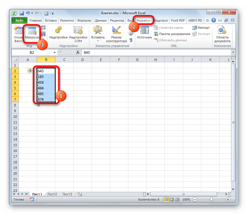
- Выделяем фрагмент на листе, который нужно преобразовать. Жмем на значок «Макросы», который расположен на вкладке «Разработчик» в группе «Код».
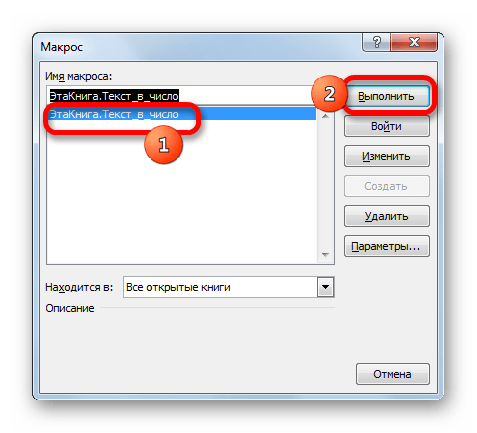
- Открывается окно записанных в вашей версии программы макросов. Находим макрос с наименованием «Текст_в_число», выделяем его и жмем на кнопку «Выполнить».
- Как видим, тут же происходит преобразование текстового выражения в числовой формат.
Урок: Как создать макрос в Экселе
Как видим, существует довольно много вариантов преобразования в Excel цифр, которые записаны в числовом варианте, в текстовый формат и в обратном направлении. Выбор определенного способа зависит от многих факторов. Прежде всего, это поставленная задача. Ведь, например, быстро преобразовать текстовое выражение с иностранными разделителями в числовое можно только использовав инструмент «Текст столбцами». Второй фактор, который влияет на выбор варианта – это объемы и частота выполняемых преобразований. Например, если вы часто используете подобные преобразования, имеет смысл произвести запись макроса. И третий фактор – индивидуальное удобство пользователя.
Before we have wrote a post to describe that how to convert number to Text string with Text Function in excel. This post will guide you how to convert number to Text using The Format Cells Command and Text to Columns wizard in excel.
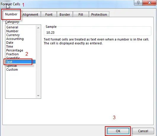
Convert Number to Text Using Format Cells Option
You also can be used the Format Cells option to change the number to Text string in excel. It may be another quick way to change the numeric value to text string in excel.
1# select the range with the numbers that you want to convert to text.
2#Right-click the selected range in the step1, and then click “Format Cells...” item from the pop-up menu list.
3# “Format Cells” window will appear.
4# Select “Text” under the Number tab and then click OK button.
Convert Number to Text Using Text to Columns wizard
1# Select the column that you want to convert numbers to text string
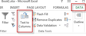
2# click on the “Text to Columns” button under DATA tab on excel ribbon.
3# “Convert Text to Columns Wizard” window will appear.
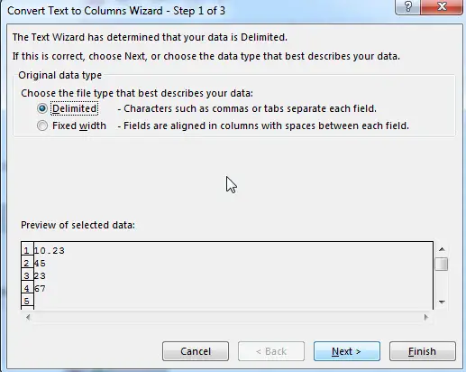
4# click “next” button through step 1 and step 2. Select “Text” radio button under step 3. Then click on “Finish” button.
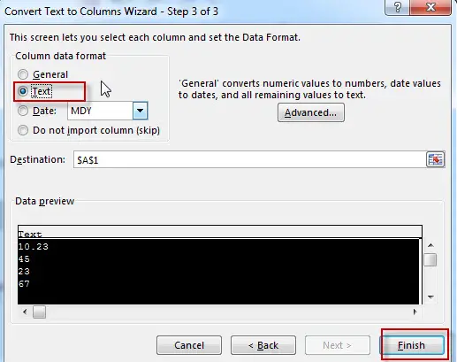
You will see that the numbers is converted to text now.
Convert Number to Text Using Concatenate Operator
We can also use another way to change the numeric value to string using Excel Concatenate operator.
The concatenation operator (&) can join together text and numbers into a single text string in excel. So if you just concatenate an empty text string (such as: “”) and a numeric value together, the returned value will be a text string. Let’s see the below example:
=""&A1
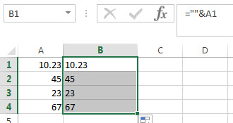
You need to enter the above excel formula in the B1 cell, then click “enter”. You will see that the numeric value in Cell A1 be changed as text string in B1.
Also read: Excel Convert numbers to Text