
For example you received a sales table in which months are displayed as numbers, and you need to convert the numbers to normal month names as below screenshot shown. Any idea? This article will introduce two solutions for you.
- Convert 1-12 to month name with formula
- Convert 1-12 to month name with Kutools for Excel

Convert 1-12 to month name with formula
Actually, we can apply the TEXT function to convert numbers (from 1 to 12) to normal month names easily in Excel. Please do as follows:
Select a blank cell next to the sales table, type the formula =TEXT(A2*29,»mmm») (Note: A2 is the first number of the Month list you will convert to month name), and then drag the AutoFill Handle down to other cells.

Now you will see the numbers (from 1 to 12) are converted to normal month names.
Convert 1-12 to month name with Kutools for Excel
As you see, the TEXT function can return month name in another cell. But if you have Kutools for Excel installed, you can apply its Operation feature to replace the numbers (from 1 to 12) with month names directly.
Kutools for Excel — Includes more than 300 handy tools for Excel. Full feature free trial 30-day, no credit card required! Get It Now
1. Select the numbers you will convert to month names in the sales table, and click Kutools > More > Operation. See screenshot:

2. In the Operation Tools dialog box, please (1) click to highlight Custom in the Operation box; (2) type the formula =TEXT(?*29,»mmm») in the Custom box; (3) check the Create formulas option; and finally (4) click the Ok button. See screenshot:

Now you will see the month names replace the selected numbers directly. See screenshot:

Related articles:
The Best Office Productivity Tools
Kutools for Excel Solves Most of Your Problems, and Increases Your Productivity by 80%
- Reuse: Quickly insert complex formulas, charts and anything that you have used before; Encrypt Cells with password; Create Mailing List and send emails…
- Super Formula Bar (easily edit multiple lines of text and formula); Reading Layout (easily read and edit large numbers of cells); Paste to Filtered Range…
- Merge Cells/Rows/Columns without losing Data; Split Cells Content; Combine Duplicate Rows/Columns… Prevent Duplicate Cells; Compare Ranges…
- Select Duplicate or Unique Rows; Select Blank Rows (all cells are empty); Super Find and Fuzzy Find in Many Workbooks; Random Select…
- Exact Copy Multiple Cells without changing formula reference; Auto Create References to Multiple Sheets; Insert Bullets, Check Boxes and more…
- Extract Text, Add Text, Remove by Position, Remove Space; Create and Print Paging Subtotals; Convert Between Cells Content and Comments…
- Super Filter (save and apply filter schemes to other sheets); Advanced Sort by month/week/day, frequency and more; Special Filter by bold, italic…
- Combine Workbooks and WorkSheets; Merge Tables based on key columns; Split Data into Multiple Sheets; Batch Convert xls, xlsx and PDF…
- More than 300 powerful features. Supports Office / Excel 2007-2021 and 365. Supports all languages. Easy deploying in your enterprise or organization. Full features 30-day free trial. 60-day money back guarantee.
")
Office Tab Brings Tabbed interface to Office, and Make Your Work Much Easier
- Enable tabbed editing and reading in Word, Excel, PowerPoint, Publisher, Access, Visio and Project.
- Open and create multiple documents in new tabs of the same window, rather than in new windows.
- Increases your productivity by 50%, and reduces hundreds of mouse clicks for you every day!
")
Comments (16)
Rated 4.5 out of 5
·
2 ratings
Содержание
- How to Convert Month Number to Month Name in Excel
- How to Convert a Given Number to Month Name in Excel
- Using the TEXT Function to Convert Month Number to Month Name in Excel
- Using the CHOOSE Function to Convert Month Number to Month Name in Excel
- How to Convert a Given Date to Month Name
- Using the TEXT Function to Convert a Date to Month Name in Excel
- Using the CHOOSE Function to Convert a Date to Month Name in Excel
- Using the Format Cells Feature to Convert a Date to Month Name in Excel
- How to Convert Date to Month and Year in Excel
- The Sample Data
- Convert Date to Month and Year using the MONTH and YEAR function
- Convert Date to Month and Year using the TEXT Function
- Format Codes for Year:
- Format Codes for Month of the Year:
- Convert Date to Month and Year using Number Formatting
How to Convert Month Number to Month Name in Excel
When working with date-related data, there might be instances where you need to convert a number to its corresponding month. There might also be instances when you might want to extract the month name corresponding to a given date.
In this tutorial we will discuss two ways to convert a month number to a month name in Excel:
- Using the TEXT function
- Using the CHOOSE function
We will also discuss three ways to convert a given date into the corresponding month name.
- Using the TEXT function
- Using the Format Cells feature
- Using the CHOOSE function
Table of Contents
How to Convert a Given Number to Month Name in Excel
Let us first consider the case where you want to convert a month number to month names. There are two ways to accomplish this in Excel:
- using the TEXT function
- using the CHOOSE function
Let us look at each of these ways one by one.
Using the TEXT Function to Convert Month Number to Month Name in Excel
When you use just a number to denote a month (not a date or date serial number), Excel usually cannot make sense of it. It does not understand that the number 1 means January, 2 means February, and so on.
So we will need to convert the number to a format that Excel understands. This can be done with the help of the TEXT function.
Let’s say you have the number 5 in cell A2 and you want to convert it to the corresponding month name. You could use the TEXT function as follows:
But that would not give you the exact month you are looking for. This is because Excel considers the number 1 as day 1, number 2 as day 2, etc. So any number between 1 and 31 will correspond to a day in the month of January.
Therefore, if you want to find out the month corresponding to a number, you can multiply the number by 29, so that we get the number corresponding to a day in that month.
For example, if you multiply 5 by 29, you get 145, which can be any day in the 5th month of the year. The 5th month of the year is May, so the above function returns the month name, May.
The following screenshot shows how the above formula works with different number inputs:

Note: If you want the shorter version of the month name, like Jan, Feb, etc. then you can use the string parameter “mmm” instead of “mmmm”:

Using the CHOOSE Function to Convert Month Number to Month Name in Excel
The CHOOSE function provides another great way to convert a month number to the month name in Excel.
The Excel CHOOSE function returns a value from a list using a given position or index. The syntax for the CHOOSE function is as follows:
- index_num is the index or position of the value you want to choose. It can be an integer value between 1 and 254.
- value1 is the value corresponding to the first index.
- value2, value3, etc. are the values corresponding to the subsequent indices. So value2 corresponds to the second index, and so on.
This makes it really easy to assign month names to numbers, since they follow a sequence. You can enter the month names you want to return as values in the CHOOSE function, after the first argument. The first argument can specify a month number or a reference to the cell containing the month number.
To convert a month number in cell reference A2, for example, we can use the CHOOSE function as shown below:
The CHOOSE function will then use the month number specified in cell A2, say n, to extract and return the nth value in the list.
The following screenshot shows how the above formula works with different number inputs:

This method is more flexible than the first method (using the TEXT function) because it allows us to map the month number to any set of values you want.
You can customize the month values (month names) inside the CHOOSE function to any form. They could be abbreviated, not abbreviated, or even in a different language.
You can see from the screenshot below different ways of using the CHOOSE function to customize month names:

How to Convert a Given Date to Month Name
Now, what if, instead of a month number, you are given a date, and you need to extract the month name from it?
In that case, all you need to do is to replace the cell reference in both the above methods with the MONTH Function.
Using the TEXT Function to Convert a Date to Month Name in Excel
Let’s say you have the date 04/06/2021 in cell A2. You can then use the TEXT function to extract the month name from the date as follows:
This will display the full month’s name corresponding to the date.

Note: If you want the shorter version of the month name, like Jan, Feb, etc. then you can use the string parameter “mmm” instead of “mmmm”:

Using the CHOOSE Function to Convert a Date to Month Name in Excel
If you want to convert the date, which is in a cell, say A2, then you can use the CHOOSE function to display the month corresponding to the date, as follows:
Note: As mentioned before, you can use the CHOOSE function to display the month in any custom format that you want, as long as you have the MONTH function with the cell reference to the date as the first parameter.
Using the Format Cells Feature to Convert a Date to Month Name in Excel
A third technique to convert a date to a month name is using the Format Cells feature. This technique is ideal and quick if you want to convert the date in place, instead of having to use a separate cell with a function.
To use this method, follow the steps below:
- Select all the cells containing the dates you want to convert.
- Right-click your selection and click on ‘Format cells’ from the context menu that appears.

- This will open the ‘Format Cells’ dialog box. Select the ‘Number’ tab.
- From the Category list on the left side, select the ‘Custom’ option.
- In the input box just under ‘Type’ (on the right side of the dialog box), type the format “mmmm” if you want the full month name, or “mmm” if you want the abbreviated version of the month name.
- Click OK.
- Your selected date values should now be replaced with the corresponding month names.


In this tutorial, I showed you two ways to convert a month number to a month name.
I also showed you how to extract the month names from a given date value.
I hope you found the tutorial helpful.
Other Excel tutorials you may also like:
Источник
How to Convert Date to Month and Year in Excel
Whenever you enter a date in a cell, Excel automatically recognizes the format and converts the cell to a date cell.
So, Excel knows which part of the date you entered is the month, which is the year and which is the day.
This can be quite helpful in many ways. One particular benefit of this capability of Excel is that it lets you display the date in any format you want. It even lets you extract parts of the date that you need.
For example, you might find the day part of the date irrelevant and just need to display the month and year.
Since Excel already understands your date, you can easily extract just the month and year and display it in any format you like.
In this tutorial, we are going to see three ways in which you can convert date to month and year in Excel.
Table of Contents
The Sample Data
Throughout this tutorial, we are going to be using the following set of dates. We will be converting these dates to month and year in Excel:

When working with dates, first and foremost, it is important to recognize the original format your Excel dates are in. For example, in the US format, dates usually begin with the month and end with the year (mm/dd/yyyy).
In the UK and other countries, dates begin with the day and end with the year (dd/mm/yyyyy). In still other places like China, Iran, and Korea, the order is completely flipped (yyyy/mm/dd).
Depending on your computer’s date settings Excel will treat parts of your date differently. So when entering the date, make sure you check the format and enter the date in the correct order. You don’t want the date 2/10 to be treated as October, the 2nd instead of February, the 10th!
Convert Date to Month and Year using the MONTH and YEAR function
The MONTH and YEAR functions can help you extract just the month or year respectively from a date cell. In order for this method to work, the original date (on which you want to operate) must be a valid Excel date. If not, then both these functions will return a #VALUE error.
Let’s see how you can extract the month from our sample data:
- Click on a blank cell where you want the month to be displayed (B2)
- Type: =MONTH, followed by an opening bracket (.
- Click on the first cell containing the original date (A2).
- Add a closing bracket )
- Press the Return key.
- This should display the month of the year corresponding to the original date. Copy this to the rest of the cells in the column by dragging down the fill handle or double-clicking on it.

You will see column B populated by the month of the year for all the dates of column A.

Now let’s see how you can extract the year from the same dataset:
- Click on a blank cell where you want the year to be displayed (C2)
- Type: =YEAR, followed by an opening bracket (.
- Click on the first cell containing the original date (A2).
- Add a closing bracket )
- Press the Return key.
- This should display the year corresponding to the original date. Copy this to the rest of the cells in the column by dragging down the fill handle or double-clicking on it.

You will see column C populated by the year corresponding to all the dates of column A.

Now let’s see how you can combine the results of the two to display both month and year in a nice format.
Let us say you want to display both month and year as “2-2018” for the date “02/10/2018”, and want to follow this pattern for all the dates.
- Click on a blank cell where you want the new date format to be displayed (D2)
- Type the formula: =B2 & “-“ & C2. Alternatively, you can type: =MONTH(A2) & “-” & YEAR(A2).
- Press the Return key.
- This should display the original date in our required format. Copy this to the rest of the cells in the column by dragging down the fill handle or double-clicking on it.

Now all your cells in column D2 have the new format:

Alternatively, if you want to display your month and year as 2/2018 instead, you only need to replace the “-“ in-between with a “/”. In this way, you can display the month and year in any format that you like.

Finally, if you want to just keep the converted values and want to remove the original dates and any intermediate columns that you created you need to first convert the formula results into constant values.
For this, copy the cells of column D and paste them as values in the same column (Right-click and select Paste Options->Values from the Popup menu). Now you can go ahead and delete columns A to C. You will be left with only the converted values that have the month and year.

Although this is quite an easy and intuitive way to convert dates to months and years, it is a less popular method. This is because this method does not provide a lot of flexibility compared to the other two methods we will show next.
Convert Date to Month and Year using the TEXT Function
The TEXT function in Excel converts any numeric value (like date, time, and currency) into text with a specified format.
The syntax of the TEXT function is:
= TEXT (value, format_code)
- value is the numeric value or reference to the cell that you want to convert
- format_code is the format you want to convert the cell into
In the above example, the TEXT function applies the format_code that you specified on the value and returns a text string with that format. For example, if you have a date “2/10/2018” in cell A2, then =TEXT(A2, “mm/yyyy”) will return “02/2018”
There are a number of format codes that you can use. We have enlisted below the basic building blocks for the format codes:
Format Codes for Year:
You can use the following two basic format codes to represent year values:
- yy – two-digit representation of year (e.g. 20 or 12)
- yyyy – four-digit representation of year (e.g. 2020 or 2012)
So, if you apply =TEXT(A2, yy) in our example dataset, it will return “18”.
If you apply =TEXT(A2, yyyy), then it will return “2018”.
Format Codes for Month of the Year:
You can use the following four basic format codes to represent month values:
- m – one or two-digit representation of the month (eg; 8 or 12)
- mm – two-digit representation of the month (eg; 08 or 12)
- mmm – month abbreviated in three letters (eg: Aug or Dec)
- mmmm – month expressed with the full name (eg: August or December)
So, if you apply =TEXT(A2, m) in our example dataset, it will return “2”.
- If you apply =TEXT(A2, mm), then it will return “02”.
- If you apply =TEXT(A2, mmm), then it will return “Feb”.
- If you apply =TEXT(A2, mmmm), then it will return “February”.
Let us see how we can apply the TEXT function to our sample dataset to convert all the dates to different formats.
We will first see how to convert the dates in column A to the format shown in column B in the image below:

Below are the steps to change the date format and only get month and year using the TEXT function:
- Click on a blank cell where you want the new date format to be displayed (B2)
- Type the formula:
- Press the Return key.
- This should display the original date in our required format. Copy this to the rest of the cells in the column by dragging down the fill handle or double-clicking on it.
- Copy this column’s formula results by pressing CTRL+C or Cmd+C (if you’re on a Mac).
- Right-click on the column and form the popup menu that appears, press Paste Values from the Paste Options.
- This will store the formula results as permanent values in the same column. Now you can go ahead and remove column A if you want to.


The format code that you put in the formula (at step 2) will vary according to the format you want your month and year to appear in. Here are the format codes along with the type of result you will get when applied to cell A2:
| Function | Result |
| =TEXT(A2, “mm/yy”) | 02/18 |
| =TEXT(A2, “mm-yy”) | 02-18 |
| =TEXT(A2, “mm-yyyy”) | 02-2018 |
| =TEXT(A2, “mmm, yyyy”) | Feb, 2018 |
| =TEXT(A2, “mmmm, yyyy”) | February, 2018 |

So you see, you can use the TEXT function to convert your dates to any format of your choice. All you need to do is change the format code according to your requirement.
Note: Using this formula, your date gets converted to a text format. If you want to convert it back to a date format, you need to use the Format Cells feature.
Convert Date to Month and Year using Number Formatting
Excel’s Format Cell feature is a versatile one that lets you perform different types of formatting through a single dialog box.
Here’s how you can convert the dates in our sample dataset to different formats.
- Select all the cells containing the dates that you want to convert (A2:A6).
- Right-click on your selection and select Format Cells from the popup menu that appears. Alternatively, you can select the dialog box launcher in the Number group under the Home tab.
- This will open the Format Cells dialog box. Click on the Number tab
- Under Category on the left side of the box, select the Date option.
- This will display a number of formatting options for date on the right side.
- Select the format that you want. For example, if you want to display the first date in the format “Feb-18”, then select the matching format option.
- If you don’t find an option for the format you want to use, then you can use the Custom option from the Category list on the left. This lets you convert the cell to a custom format.
- Look if your format is available among the date format codes under Type. If not, you can type in your format code in the input box just below Type. So, if you want to display the first month in the format “2/18”, then type “m/yy”.
- Click OK to close the Format Cells dialog box.


All your selected cells should now be formatted to your required format.

This method differs from the previous one (using the TEXT function) in four ways:
- With this method, you can perform the operation directly on the original cells.
- You can get your conversion done in one go. So you don’t need to have a separate cell to enter the formula, then paste by value and then delete the original cells (as you would need to if using the TEXT function).
- This method changes just the format of the original date, the underlying date, however, remains the same. So if you want to later recover the original date value (along with the day), you can easily access it. With the TEXT function method, however, the original date value is lost because the conversion changes the entire value of the date.
- The results you get from using this method are of type Date, rather than Text, so you can perform date operations on them directly without having to convert them.
These were three ways in which you can convert date to month and year in Excel. Using these you can convert your date to any format you need.
We hope you found our methods useful and that you will apply it to your own Excel data.
Other Excel tutorials you may like:
Источник
OBJECTS
Worksheets: The Worksheets object represents all of the worksheets in a workbook, excluding chart sheets.
Range: The Range object is a representation of a single cell or a range of cells in a worksheet.
PREREQUISITES
Worksheet Name: Have a worksheet named Analysis.
Number Rage: In this example we are converting numbers in range («B5:B16») into month names. Therefore, if you are using this exact VBA code you will need to capture all the numbers in range («B5:B16») that you want to convert into a month name.
ADJUSTABLE PARAMETERS
Output Range: Select the output range by changing the cell reference («C5») in the VBA code to any cell in the worksheet, that doesn’t conflict with the formula.
Number Rage: Select the range that captures the numbers that you want to convert into month names by changing the range reference («B5:B16») in the VBA code to any range in the worksheet that doesn’t conflict with the formula. If you change the number or location of rows then you will need to change the parameters that is driving the For Loop. In this case its the values that we have nominated for x, which are from 5 to 16.
Функции и формулы для преобразования номера в название месяца
Время от времени возникает необходимость изменить порядковый номер месяца на название и наоборот (например, 3 на «Март» или «Октябрь» на 10).
Сначала рассмотрим, каким способом изменить номер месяца его название. А после речь пойдет о том, как выполнить обратный процесс, то есть изменить название на соответствующий ему порядковый номер.
Изменение порядкового номера месяца на его название в Excel
Первый способ, который пришел мне на ум, это просто составить список ячеек с последовательными названиями месяцев, а затем использовать функцию:
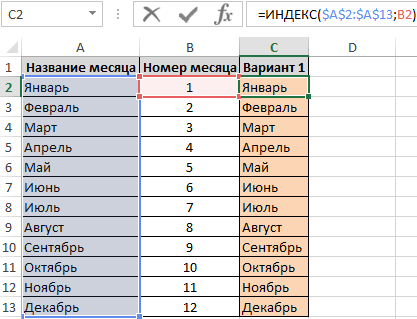
=ИНДЕКС($A$2:$A$13;B2)
где $A$2:$A$13 – это, конечно, диапазон с названиями месяцев, а B2 — ячейка с порядковым номером в году, для которого мы ищем его название.
По схожему принципу с функцией ИНДЕКС работает другая функция, которую вы можете использовать — ВЫБОР. Разница состоит в том, что она не использует ячейки листа, в которых хранятся названия месяцев. Названия месяцев просто даем в качестве аргумента функции.
Функция ВЫБОР принимает в качестве аргументов номер индекса (который определяет какой из элементов в списке значений вернуть в качестве результата) и список значений. Интересующиеся подробностями, конечно же, могут скачать файл с примерами.
Если в качестве списка значений указать названия месяцев (по очередности), а в качестве индекса — ячейку с номером месяца, то функция вернет соответствующее ему название для каждого заданного числа.
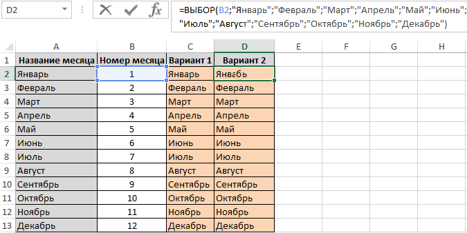
Вариант2 автономный и более удобный для использования формулы на разных листах или рабочих книга без применения внешних ссылок.
Примеры как получить название месяца из даты в Excel
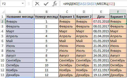
Подобно тому как показано выше, в случае, когда необходимо «вытянуть» название месяца из даты, необходимо воспользоваться помощью функции МЕСЯЦ.
Если у вас есть список с датами и нужно «вытянуть» из них название месяцев, то функция ИНДЕКС в приведенном выше виде выдаст ошибку. Если вы хотите, чтобы формула работала правильно, необходимо при помощи функции МЕСЯЦ «вытянуть» номер месяца из ячейки с датой. Формула будет выглядеть следующим образом:
=ИНДЕКС($A$2:$A$13;МЕСЯЦ(E2))
Еще один способ (возможно, самый удобный) — использовать функцию ТЕКСТ (все, что делает функция ТЕКСТ, это преобразует числовое значение в текст с соответствующим форматированием).
Если у вас есть список с датами и нужно «вытянуть» из них название месяцев, просто введите:
=ТЕКСТ(E2;»mmmm»)
где E2 – это, конечно, ячейка с датой.
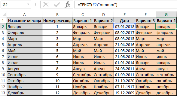
Если вы работаете только с числами (1-12), функция в приведенной выше форме будет работать неправильно. Вы должны помнить, что число 1 для Excelя это 1 января 1900 года, число 2 — 2 января 1900 года и так далее. Это все тот же месяц — январь. Поэтому ТЕКСТ(E2;»ММММ») возвращает «Январь» для каждого номера месяца.
Однако вы можете легко изменить последовательные числа на номера месяцев. Например, вы можете умножить каждое число на среднее количество дней в месяце (30).
Формула функции:
=ТЕКСТ(B2*30;»mmmm»)
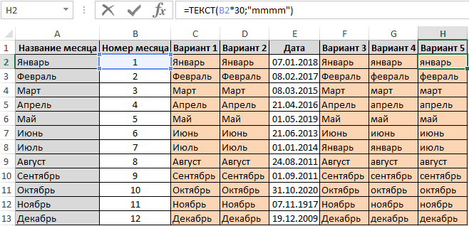
будет работать правильно, и в качестве результата вернет названия месяцев.
Как преобразовать название месяца в порядковый номер
Теперь будем преобразовывать обратно – имя месяца в соответствующий ему порядковый номер в году.
Пример1. Формула первая:
=МЕСЯЦ(ДАТАЗНАЧ(A2&»1″))

Значение Декабрь1 Excel автоматически преобразует в дату дек.01. Далее функция ДАТАЗНАЧ преобразует дату в число после с помощью функции МЕСЯЦ мы получаем порядковый номер в году для текущего названия месяца. По сути формулу можно упростить:
=МЕСЯЦ(A2&»1″)
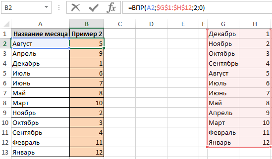
Пример2. Формула вторая:
=ВПР(A2;$G$1:$H$12;2;0)
Пример3. Формула третья:
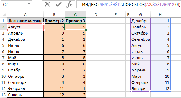
Наиболее оптимальным вариантом является лаконичная формула =МЕСЯЦ(A2&»1″). В ней не нужно резервировать названия месяцев и присваивать им соответственные порядковые номера. К тому же в ней используется всего лишь одна функция.
When working with date-related data, there might be instances where you need to convert a number to its corresponding month. There might also be instances when you might want to extract the month name corresponding to a given date.
In this tutorial we will discuss two ways to convert a month number to a month name in Excel:
- Using the TEXT function
- Using the CHOOSE function
We will also discuss three ways to convert a given date into the corresponding month name.
- Using the TEXT function
- Using the Format Cells feature
- Using the CHOOSE function
Let us first consider the case where you want to convert a month number to month names. There are two ways to accomplish this in Excel:
- using the TEXT function
- using the CHOOSE function
Let us look at each of these ways one by one.
Using the TEXT Function to Convert Month Number to Month Name in Excel
When you use just a number to denote a month (not a date or date serial number), Excel usually cannot make sense of it. It does not understand that the number 1 means January, 2 means February, and so on.
So we will need to convert the number to a format that Excel understands. This can be done with the help of the TEXT function.
Let’s say you have the number 5 in cell A2 and you want to convert it to the corresponding month name. You could use the TEXT function as follows:
=TEXT(A2, “mmmm”)
But that would not give you the exact month you are looking for. This is because Excel considers the number 1 as day 1, number 2 as day 2, etc. So any number between 1 and 31 will correspond to a day in the month of January.
Therefore, if you want to find out the month corresponding to a number, you can multiply the number by 29, so that we get the number corresponding to a day in that month.
For example, if you multiply 5 by 29, you get 145, which can be any day in the 5th month of the year. The 5th month of the year is May, so the above function returns the month name, May.
The following screenshot shows how the above formula works with different number inputs:
Note: If you want the shorter version of the month name, like Jan, Feb, etc. then you can use the string parameter “mmm” instead of “mmmm”:
Using the CHOOSE Function to Convert Month Number to Month Name in Excel
The CHOOSE function provides another great way to convert a month number to the month name in Excel.
The Excel CHOOSE function returns a value from a list using a given position or index. The syntax for the CHOOSE function is as follows:
=CHOOSE (index_num, value1, [value2], ...)
Here,
- index_num is the index or position of the value you want to choose. It can be an integer value between 1 and 254.
- value1 is the value corresponding to the first index.
- value2, value3, etc. are the values corresponding to the subsequent indices. So value2 corresponds to the second index, and so on.
This makes it really easy to assign month names to numbers, since they follow a sequence. You can enter the month names you want to return as values in the CHOOSE function, after the first argument. The first argument can specify a month number or a reference to the cell containing the month number.
To convert a month number in cell reference A2, for example, we can use the CHOOSE function as shown below:
=CHOOSE(A2,"Jan","Feb","Mar","Apr","May","Jun","Jul","Aug","Sep","Oct","Nov","Dec")
The CHOOSE function will then use the month number specified in cell A2, say n, to extract and return the nth value in the list.
The following screenshot shows how the above formula works with different number inputs:
This method is more flexible than the first method (using the TEXT function) because it allows us to map the month number to any set of values you want.
You can customize the month values (month names) inside the CHOOSE function to any form. They could be abbreviated, not abbreviated, or even in a different language.
You can see from the screenshot below different ways of using the CHOOSE function to customize month names:
One good thing that I like about this method is that you can customize it easily for the calendar year as well as the financial year. For example, if I’m working with financial data and I want 1 to represent April and 2 to represent May (as so on), then I can easily tweak this formula
How to Convert a Given Date to Month Name
Now, what if, instead of a month number, you are given a date, and you need to extract the month name from it?
In that case, all you need to do is to replace the cell reference in both the above methods with the MONTH Function.
Using the TEXT Function to Convert a Date to Month Name in Excel
Let’s say you have the date 04/06/2021 in cell A2. You can then use the TEXT function to extract the month name from the date as follows:
=TEXT(MONTH(A2),”mmmm”)
This will display the full month’s name corresponding to the date.
Note: If you want the shorter version of the month name, like Jan, Feb, etc. then you can use the string parameter “mmm” instead of “mmmm”:
Using the CHOOSE Function to Convert a Date to Month Name in Excel
If you want to convert the date, which is in a cell, say A2, then you can use the CHOOSE function to display the month corresponding to the date, as follows:
=CHOOSE(MONTH(A2),"Jan","Feb","Mar","Apr","May","Jun","Jul","Aug","Sep","Oct","Nov","Dec")
Note: As mentioned before, you can use the CHOOSE function to display the month in any custom format that you want, as long as you have the MONTH function with the cell reference to the date as the first parameter.
Using the Format Cells Feature to Convert a Date to Month Name in Excel
A third technique to convert a date to a month name is using the Format Cells feature. This technique is ideal and quick if you want to convert the date in place, instead of having to use a separate cell with a function.
To use this method, follow the steps below:
- Select all the cells containing the dates you want to convert.
- Right-click your selection and click on ‘Format cells’ from the context menu that appears.

- This will open the ‘Format Cells’ dialog box. Select the ‘Number’ tab.

- From the Category list on the left side, select the ‘Custom’ option.
- In the input box just under ‘Type’ (on the right side of the dialog box), type the format “mmmm” if you want the full month name, or “mmm” if you want the abbreviated version of the month name.
- Click OK.
- Your selected date values should now be replaced with the corresponding month names.

One great thing about this method is that it is not going to change the value in the cell. It will only change the way that values displayed in the cell. For example, if after applying this custom number formatting method, your date may be shown as April or May (or whatever the month name is), but in the backend, it would still hold the full date and you can use it in calculations.
In this tutorial, I showed you two ways to convert a month number to a month name.
I also showed you how to extract the month names from a given date value.
I hope you found the tutorial helpful.
Other Excel tutorials you may also like:
- How to Convert Date to Month and Year in Excel (3 Easy Ways)
- How to Convert Date to Day of Week in Excel (3 Easy Ways)
- How to Convert Serial Numbers to Date in Excel
- How to Add Days to a Date in Excel
- Why are Dates Shown as Hashtags in Excel? Easy Fix!
- How to Convert Days to Years in Excel (Simple Formulas)
- How to Convert Month Name to Number in Excel?
- Find Last Monday of the Month Date in Excel
- How to Remove Year from Date in Excel?