
В Excel мы можем пронумеровать ячейки с помощью числовых рядов, таких как 1, 2, 3… с помощью дескриптора автозаполнения, но как вы можете пронумеровать ячейки с помощью букв алфавита A, B, C…? В этом руководстве я расскажу о некоторых способах выполнения этой работы в Excel.
Нумерация ячеек буквой алфавита с формулой
Нумерация ячеек буквой алфавита с кодом VBA
Нумерация ячеек с с Kutools for Excel![]()
Нумерация ячеек буквой алфавита с формулой
1. Введите все буквы, которые вы хотите использовать для нумерации ячеек в списке, рядом с ячейками, которые вы хотите пронумеровать.
2. Выберите ячейку, которая находится рядом с буквами и содержимым ячейки, которое вы хотите пронумеровать, введите эту формулу. = A1 & «.» & B1перетащите дескриптор заполнения вниз, чтобы заполнить формулой все нужные ячейки.
Нумерация ячеек буквой алфавита с кодом VBA
Если вы знакомы с кодами макросов, вы можете сделать следующее:
1. Нажмите Alt + F11 ключи для включения Microsoft Visual Basic для приложений окно. Нажмите Вставить > Модули.
2. Скопируйте и вставьте приведенный ниже код в Модули скрипты.
VBA: нумерация буквой A
Sub Prefix_A()
'UpdatebyExtendoffice20180828
Dim xRg As Range
Dim xStrPrefix As String
xStrPrefix = "A."
On Error Resume Next
Application.ScreenUpdating = False
For Each xRg In Selection
    If xRg.Value <> "" Then
        xRg.Value = xStrPrefix & xRg.Value
    End If
Next
Application.ScreenUpdating = True
End Sub
3. Затем повторите вставку кода и измените A на B, C или D, как вам нужно.
4. Сохраните код и закройте Microsoft Visual Basic для приложений окно.
5. Выберите ячейки, которые нужно пронумеровать с помощью A, и нажмите Застройщик > Макрос.
6. в Макрос диалоговом окне выберите код Префикс_A и нажмите Run.
7. Выборка пронумерована A.
8. Повторите шаги 5 и 6 для нумерации ячеек определенной буквой по мере необходимости.
Нумерация ячеек с Kutools for Excel
Если у вас есть Kutools for Excel, вы можете быстро нумеровать ячейки.
После установки Kutools for Excel, пожалуйста, сделайте следующее:(Бесплатная загрузка Kutools for Excel Сейчас!)
Выберите ячейки, которые хотите пронумеровать, затем нажмите Кутулс > Вставить > Вставить нумерацию, выберите нужный вам тип.

Затем к ячейкам была добавлена нумерация.

Просмотр и редактирование нескольких книг Excel / документов Word с вкладками в Firefox, Chrome, Internet Explore 10! |
|
Возможно, вы знакомы с просмотром нескольких веб-страниц в Firefox / Chrome / IE и возможностью переключения между ними, легко щелкая соответствующие вкладки. Здесь вкладка Office поддерживает аналогичную обработку, что позволяет вам просматривать несколько книг Excel или документов Word в одном окне Excel или Word и легко переключаться между ними, щелкая их вкладки. Нажмите бесплатно 30-дневная пробная версия Office Tab! |
 |
Лучшие инструменты для работы в офисе
Kutools for Excel Решит большинство ваших проблем и повысит вашу производительность на 80%
- Снова использовать: Быстро вставить сложные формулы, диаграммы и все, что вы использовали раньше; Зашифровать ячейки с паролем; Создать список рассылки и отправлять электронные письма …
- Бар Супер Формулы (легко редактировать несколько строк текста и формул); Макет для чтения (легко читать и редактировать большое количество ячеек); Вставить в отфильтрованный диапазон…
- Объединить ячейки / строки / столбцы без потери данных; Разделить содержимое ячеек; Объединить повторяющиеся строки / столбцы… Предотвращение дублирования ячеек; Сравнить диапазоны…
- Выберите Дубликат или Уникальный Ряды; Выбрать пустые строки (все ячейки пустые); Супер находка и нечеткая находка во многих рабочих тетрадях; Случайный выбор …
- Точная копия Несколько ячеек без изменения ссылки на формулу; Автоматическое создание ссылок на несколько листов; Вставить пули, Флажки и многое другое …
- Извлечь текст, Добавить текст, Удалить по позиции, Удалить пробел; Создание и печать промежуточных итогов по страницам; Преобразование содержимого ячеек в комментарии…
- Суперфильтр (сохранять и применять схемы фильтров к другим листам); Расширенная сортировка по месяцам / неделям / дням, периодичности и др .; Специальный фильтр жирным, курсивом …
- Комбинируйте книги и рабочие листы; Объединить таблицы на основе ключевых столбцов; Разделить данные на несколько листов; Пакетное преобразование xls, xlsx и PDF…
- Более 300 мощных функций. Поддерживает Office/Excel 2007-2021 и 365. Поддерживает все языки. Простое развертывание на вашем предприятии или в организации. Полнофункциональная 30-дневная бесплатная пробная версия. 60-дневная гарантия возврата денег.
")
Вкладка Office: интерфейс с вкладками в Office и упрощение работы
- Включение редактирования и чтения с вкладками в Word, Excel, PowerPoint, Издатель, доступ, Visio и проект.
- Открывайте и создавайте несколько документов на новых вкладках одного окна, а не в новых окнах.
- Повышает вашу продуктивность на 50% и сокращает количество щелчков мышью на сотни каждый день!
")
Комментарии (1)
Оценок пока нет. Оцените первым!
Содержание
- Convert numbers into words
- Create the SpellNumber function to convert numbers to words
- Use the SpellNumber function in individual cells
- Save your SpellNumber function workbook
- MS Excel 2016: How to Change Column Headings from Numbers to Letters
- How to convert column number to letter in Excel
- How to convert column number into alphabet (single-letter columns)
- How to convert Excel column number to letter (any column)
- Get column letter from column number using custom function Custom function
- How to get column letter of certain cell
- How to get column letter of the current cell
- How to create dynamic range reference from column number
- How to change column number with letter in Microsoft Excel
Convert numbers into words
Excel doesn’t have a default function that displays numbers as English words in a worksheet, but you can add this capability by pasting the following SpellNumber function code into a VBA (Visual Basic for Applications) module. This function lets you convert dollar and cent amounts to words with a formula, so 22.50 would read as Twenty-Two Dollars and Fifty Cents. This can be very useful if you’re using Excel as a template to print checks.
If you want to convert numeric values to text format without displaying them as words, use the TEXT function instead.
Note: Microsoft provides programming examples for illustration only, without warranty either expressed or implied. This includes, but is not limited to, the implied warranties of merchantability or fitness for a particular purpose. This article assumes that you are familiar with the VBA programming language, and with the tools that are used to create and to debug procedures. Microsoft support engineers can help explain the functionality of a particular procedure. However, they will not modify these examples to provide added functionality, or construct procedures to meet your specific requirements.
Create the SpellNumber function to convert numbers to words
Use the keyboard shortcut, Alt + F11 to open the Visual Basic Editor (VBE).
Note: You can also access the Visual Basic Editor by showing the Developer tab in your ribbon.
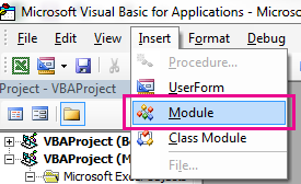
Click the Insert tab, and click Module.
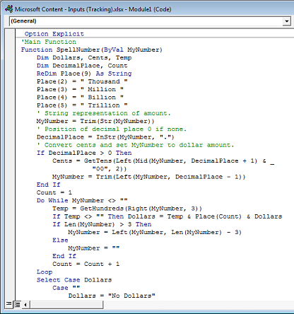
Copy the following lines of code.
Note: Known as a User Defined Function (UDF), this code automates the task of converting numbers to text throughout your worksheet.
Paste the lines of code into the Module1 (Code) box.
Press Alt + Q to return to Excel. The SpellNumber function is now ready to use.
Note: This function works only for the current workbook. To use this function in another workbook, you must repeat the steps to copy and paste the code in that workbook.
Use the SpellNumber function in individual cells
Type the formula =SpellNumber( A1) into the cell where you want to display a written number, where A1 is the cell containing the number you want to convert. You can also manually type the value like =SpellNumber(22.50).
Press Enter to confirm the formula.
Save your SpellNumber function workbook
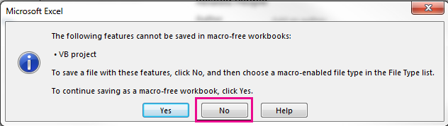
Excel cannot save a workbook with macro functions in the standard macro-free workbook format (.xlsx). If you click File > Save. A VB project dialog box opens. Click No.
You can save your file as an Excel Macro-Enabled Workbook (.xlsm) to keep your file in its current format.
Click File > Save As.
Click the Save as type drop-down menu, and select Excel Macro-Enabled Workbook.
Источник
MS Excel 2016: How to Change Column Headings from Numbers to Letters
This Excel tutorial explains how to change column headings from numbers (1, 2, 3, 4) back to letters (A, B, C, D) in Excel 2016 (with screenshots and step-by-step instructions).
See solution in other versions of Excel :
Question: In Microsoft Excel 2016, my Excel spreadsheet has numbers for both rows and columns. How do I change the column headings back to letters such as A, B, C, D?
Answer: Traditionally, column headings are represented by letters such as A, B, C, D. If your spreadsheet shows the columns as numbers, you can change the headings back to letters with a few easy steps.
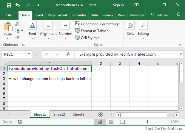
In the example below, the column headings are numbered 1, 2, 3, 4 instead of the traditional A, B, C, D values that you normally see in Excel. When the column headings are numeric values, R1C1 reference style is being displayed in the spreadsheet.
To change the column headings to letters, select the File tab in the toolbar at the top of the screen and then click on Options at the bottom of the menu.
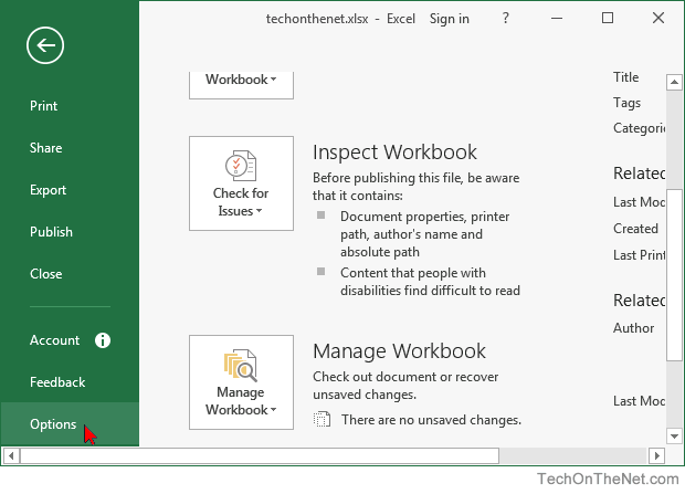
When the Excel Options window appears, click on the Formulas option on the left. Then uncheck the option called «R1C1 reference style» and click on the OK button.

Now when you return to your spreadsheet, the column headings should be letters (A, B, C, D) instead of numbers (1, 2, 3, 4).
Источник
How to convert column number to letter in Excel
 by Svetlana Cheusheva, updated on March 9, 2023
In this tutorial, we’ll look at how to change Excel column numbers to the corresponding alphabetical characters.
When building complex formulas in Excel, you may sometimes need to get a column letter of a specific cell or from a given number. This can be done in two ways: by using inbuilt functions or a custom one.
How to convert column number into alphabet (single-letter columns)
In case the column name consists of a single letter, from A to Z, you can get it by using this simple formula:
For example, to convert number 10 to a column letter, the formula is:
It’s also possible to input a number in some cell and refer to that cell in your formula:
=CHAR(64 + A2) 
How this formula works:
The CHAR function returns a character based on the character code in the ASCII set. The ASCII values of the uppercase letters of the English alphabet are 65 (A) to 90 (Z). So, to get the character code of uppercase A, you add 1 to 64; to get the character code of uppercase B, you add 2 to 64, and so on.
How to convert Excel column number to letter (any column)
If you are looking for a versatile formula that works for any column in Excel (1 letter, 2 letter and 3 letter), then you’ll need to use a bit more complex syntax:
With the column letter in A2, the formula takes this form:
=SUBSTITUTE(ADDRESS(1, A2, 4), «1», «») 
How this formula works:
First, you construct a cell address with the column number of interest. For this, supply the following arguments to the ADDRESS function:
- 1 for row_num (the row number does not really matter, so you can use any).
- A2 (the cell containing the column number) for column_num.
- 4 for abs_num argument to return a relative reference.
With the above parameters, the ADDRESS function returns the text string «A1» as the result.
As we only need a column letter, we strip the row number with the help of the SUBSTITUTE function, which searches for «1» (or whatever row number you hardcoded inside the ADDRESS function) in the text «A1» and replaces it with an empty string («»).
Get column letter from column number using custom function Custom function
If you need to convert column numbers into alphabetical characters on a regular basis, then a custom user-defined function (UDF) can save your time immensely.
The code of the function is pretty plain and straightforward:
Here, we use the Cells property to refer to a cell in row 1 and the specified column number and the Address property to return a string containing an absolute reference to that cell (such as $A$1). Then, the Split function breaks the returned string into individual elements using the $ sign as the separator, and we return element (1), which is the column letter.
Paste the code in the VBA editor, and your new ColumnLetter function is ready for use. For the detailed guidance, please see: How to insert VBA code in Excel.
From the end-user viewpoint, the function’s syntax is as simple as this:
Where col_num is the column number that you want to convert into a letter.
Your real formula can look as follows:
And it will return exactly the same results as native Excel functions discussed in the previous example: 
How to get column letter of certain cell
To identify a column letter of a specific cell, use the COLUMN function to retrieve the column number, and serve that number to the ADDRESS function. The complete formula will take this shape:
As an example, let’s find a column letter of cell C5:
=SUBSTITUTE(ADDRESS(1, COLUMN(C5), 4), «1», «»)
Obviously, the result is «C» 🙂 
How to get column letter of the current cell
To work out the letter of the current cell, the formula is almost the same as in the above example. The only difference is that the COLUMN() function is used with an empty argument to refer to the cell where the formula is:
=SUBSTITUTE(ADDRESS(1, COLUMN(), 4), «1», «») 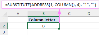
How to create dynamic range reference from column number
Hopefully, the previous examples have given you some new subjects for thought, but you may be wondering about the practical applications.
In this example, we’ll show you how to use the «column number to letter» formula for solving real-life tasks. In particular, we’ll create a dynamic XLOOKUP formula that will pull values from a specific column based on its number.
From the sample table below, suppose you wish to get a profit figure for a given project (H2) and week (H3). 
To accomplish the task, you need to provide XLOOKUP with the range from which to return values. As we only have the week number, which corresponds to the column number, we are going to convert that number to a column letter first, and then construct the range reference.
For convenience, let’s break down the whole process into 3 easy to follow steps.
- Convert a column number to a letter
With the column number in H3, use the already familiar formula to change it to an alphabetical character:
=SUBSTITUTE(ADDRESS(1, H3, 4), «1», «») 
Tip. If the number in your dataset does not match the column number, be sure to make the required correction. For example, if we had the week 1 data in column B, the week 2 data in column C, and so on, then we’d use H3+1 to get the correct column number.
To build a range reference in the form of a string, you concatenate the column letter returned by the above formula with the first and last row numbers. In our case, the data cells are in rows 3 through 8, so we are using this formula:
=SUBSTITUTE(ADDRESS(1, H3, 4), «1», «») & «3:» & SUBSTITUTE(ADDRESS(1, H3, 4), «1», «») & «8»
Given that H3 contains «3», which is converted to «C», our formula undergoes the following transformation:
And produces the string C3:C8. 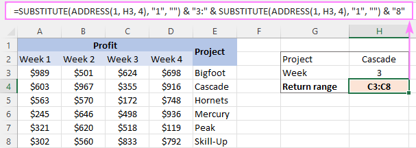
Make a dynamic range reference
To transform a text string into a valid reference that Excel can understand, nest the above formula in the INDIRECT function, and then pass it to the 3 rd argument of XLOOKUP:
=XLOOKUP(H2, E3:E8, INDIRECT(H4), «Not found») 
To get rid of an extra cell containing the return range string, you can place the SUBSTITUTE ADDRESS formula within the INDIRECT function itself:
=XLOOKUP(H2, E3:E8, INDIRECT(SUBSTITUTE(ADDRESS(1, H3, 4), «1», «») & «3:» & SUBSTITUTE(ADDRESS(1, H3, 4), «1», «») & «8»), «Not found») 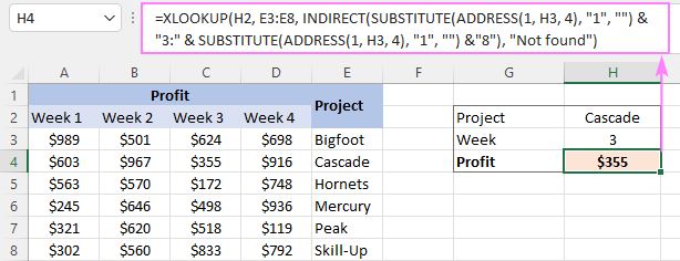
With our custom ColumnLetter function, you can get a more compact and elegant solution:
=XLOOKUP(H2, E3:E8, INDIRECT(ColumnLetter(H3) & «3:» & ColumnLetter(H3) & «8»), «Not found»)
That’s how to find a column letter from a number in Excel. I thank you for reading and look forward to seeing you on our blog next week!
Источник
How to change column number with letter in Microsoft Excel
To change in Excel column number to a letter, we need to use the «IF», «AND», «CHAR», «INT» and «MOD» functions in Microsoft Excel 2010.
Before converting the column number to a letter,let us evaluate each formula.
IF: — Checks whether a condition is met and returns one value if True and another value if False.
Syntax of “IF” function =if(logical test,[value_if_true],[value_if_false])
First the formula will perform the logical test. It will return one value if the output of the logical test is true, else it will return false.
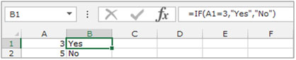
For example:Cells A2 and A3 contain the numbers 3 and 5. If the number is 3, the formula should display “Yes” otherwise “No”.
AND:- This function is used to check whether all arguments are true and returns TRUE if all arguments are TRUE. Even if one argument is false, it returns false.
The syntax of “AND” function =AND(logical1,[logical2],….)
For example:Cell A1 contains student name, B1 contains 50, and we need to check if the number is more than 40 and less than 60.
- Write the formula in cell C1
- =AND(B2>40,B2 0,A2 26,CHAR(64+INT((A2-1)/26)),»»)&CHAR(65+MOD(A2-1,26)),»»)
- Press Enter on the keyboard.
- The function will convert the number to the letter.
- To convert all the serial numbers into letters, copy the same formula by pressing the key Ctrl+Cand paste in the range B3:B15 by pressing the key Ctrl+Von your keyboard.
Note: This function will convert the serial numbers into letters till number 256. If you want to convert the numbers which are greater than 256, you will need to change the number in the formula.
Источник
Here is a quick reference for Excel column letter to number mapping. Many times I needed to find the column number associated with a column letter in order to use it in Excel Macro. For a lazy developer like me, It is very time consuming 😉 to use my Math skill to get the answer so I created this quick reference lookup for myself.
Jump to specific column list
If you are looking for a specific column, click on the following links to jump to a specific list of columns
Excel Columns A-Z
| Column Letter | Column Number |
|---|---|
| A | 1 |
| B | 2 |
| C | 3 |
| D | 4 |
| E | 5 |
| F | 6 |
| G | 7 |
| H | 8 |
| I | 9 |
| J | 10 |
| K | 11 |
| L | 12 |
| M | 13 |
| N | 14 |
| O | 15 |
| P | 16 |
| Q | 17 |
| R | 18 |
| S | 19 |
| T | 20 |
| U | 21 |
| V | 22 |
| W | 23 |
| X | 24 |
| Y | 25 |
| Z | 26 |
Excel Columns AA-AZ
| Column Letter | Column Number |
|---|---|
| AA | 27 |
| AB | 28 |
| AC | 29 |
| AD | 30 |
| AE | 31 |
| AF | 32 |
| AG | 33 |
| AH | 34 |
| AI | 35 |
| AJ | 36 |
| AK | 37 |
| AL | 38 |
| AM | 39 |
| AN | 40 |
| AO | 41 |
| AP | 42 |
| AQ | 43 |
| AR | 44 |
| AS | 45 |
| AT | 46 |
| AU | 47 |
| AV | 48 |
| AW | 49 |
| AX | 50 |
| AY | 51 |
| AZ | 52 |
Excel Columns BA-BZ
| Column Letter | Column Number |
|---|---|
| BA | 53 |
| BB | 54 |
| BC | 55 |
| BD | 56 |
| BE | 57 |
| BF | 58 |
| BG | 59 |
| BH | 60 |
| BI | 61 |
| BJ | 62 |
| BK | 63 |
| BL | 64 |
| BM | 65 |
| BN | 66 |
| BO | 67 |
| BP | 68 |
| BQ | 69 |
| BR | 70 |
| BS | 71 |
| BT | 72 |
| BU | 73 |
| BV | 74 |
| BW | 75 |
| BX | 76 |
| BY | 77 |
| BZ | 78 |
Excel Columns CA-CZ
| Column Letter | Column Number |
|---|---|
| CA | 79 |
| CB | 80 |
| CC | 81 |
| CD | 82 |
| CE | 83 |
| CF | 84 |
| CG | 85 |
| CH | 86 |
| CI | 87 |
| CJ | 88 |
| CK | 89 |
| CL | 90 |
| CM | 91 |
| CN | 92 |
| CO | 93 |
| CP | 94 |
| CQ | 95 |
| CR | 96 |
| CS | 97 |
| CT | 98 |
| CU | 99 |
| CV | 100 |
| CW | 101 |
| CX | 102 |
| CY | 103 |
| CZ | 104 |
Excel Columns DA-DZ
| Column Letter | Column Number |
|---|---|
| DA | 105 |
| DB | 106 |
| DC | 107 |
| DD | 108 |
| DE | 109 |
| DF | 110 |
| DG | 111 |
| DH | 112 |
| DI | 113 |
| DJ | 114 |
| DK | 115 |
| DL | 116 |
| DM | 117 |
| DN | 118 |
| DO | 119 |
| DP | 120 |
| DQ | 121 |
| DR | 122 |
| DS | 123 |
| DT | 124 |
| DU | 125 |
| DV | 126 |
| DW | 127 |
| DX | 128 |
| DY | 129 |
| DZ | 130 |
Excel Columns EA-EZ
| Column Letter | Column Number |
|---|---|
| EA | 131 |
| EB | 132 |
| EC | 133 |
| ED | 134 |
| EE | 135 |
| EF | 136 |
| EG | 137 |
| EH | 138 |
| EI | 139 |
| EJ | 140 |
| EK | 141 |
| EL | 142 |
| EM | 143 |
| EN | 144 |
| EO | 145 |
| EP | 146 |
| EQ | 147 |
| ER | 148 |
| ES | 149 |
| ET | 150 |
| EU | 151 |
| EV | 152 |
| EW | 153 |
| EX | 154 |
| EY | 155 |
| EZ | 156 |
Excel Columns FA-FZ
| Column Letter | Column Number |
|---|---|
| FA | 157 |
| FB | 158 |
| FC | 159 |
| FD | 160 |
| FE | 161 |
| FF | 162 |
| FG | 163 |
| FH | 164 |
| FI | 165 |
| FJ | 166 |
| FK | 167 |
| FL | 168 |
| FM | 169 |
| FN | 170 |
| FO | 171 |
| FP | 172 |
| FQ | 173 |
| FR | 174 |
| FS | 175 |
| FT | 176 |
| FU | 177 |
| FV | 178 |
| FW | 179 |
| FX | 180 |
| FY | 181 |
| FZ | 182 |
Excel Columns GA-GZ
| Column Letter | Column Number |
|---|---|
| GA | 183 |
| GB | 184 |
| GC | 185 |
| GD | 186 |
| GE | 187 |
| GF | 188 |
| GG | 189 |
| GH | 190 |
| GI | 191 |
| GJ | 192 |
| GK | 193 |
| GL | 194 |
| GM | 195 |
| GN | 196 |
| GO | 197 |
| GP | 198 |
| GQ | 199 |
| GR | 200 |
| GS | 201 |
| GT | 202 |
| GU | 203 |
| GV | 204 |
| GW | 205 |
| GX | 206 |
| GY | 207 |
| GZ | 208 |
Excel Columns HA-HZ
| Column Letter | Column Number |
|---|---|
| HA | 209 |
| HB | 210 |
| HC | 211 |
| HD | 212 |
| HE | 213 |
| HF | 214 |
| HG | 215 |
| HH | 216 |
| HI | 217 |
| HJ | 218 |
| HK | 219 |
| HL | 220 |
| HM | 221 |
| HN | 222 |
| HO | 223 |
| HP | 224 |
| HQ | 225 |
| HR | 226 |
| HS | 227 |
| HT | 228 |
| HU | 229 |
| HV | 230 |
| HW | 231 |
| HX | 232 |
| HY | 233 |
| HZ | 234 |
Excel Columns IA-IZ
| Column Letter | Column Number |
|---|---|
| IA | 235 |
| IB | 236 |
| IC | 237 |
| ID | 238 |
| IE | 239 |
| IF | 240 |
| IG | 241 |
| IH | 242 |
| II | 243 |
| IJ | 244 |
| IK | 245 |
| IL | 246 |
| IM | 247 |
| IN | 248 |
| IO | 249 |
| IP | 250 |
| IQ | 251 |
| IR | 252 |
| IS | 253 |
| IT | 254 |
| IU | 255 |
| IV | 256 |
| IW | 257 |
| IX | 258 |
| IY | 259 |
| IZ | 260 |
Excel Columns JA-JZ
| Column Letter | Column Number |
|---|---|
| JA | 261 |
| JB | 262 |
| JC | 263 |
| JD | 264 |
| JE | 265 |
| JF | 266 |
| JG | 267 |
| JH | 268 |
| JI | 269 |
| JJ | 270 |
| JK | 271 |
| JL | 272 |
| JM | 273 |
| JN | 274 |
| JO | 275 |
| JP | 276 |
| JQ | 277 |
| JR | 278 |
| JS | 279 |
| JT | 280 |
| JU | 281 |
| JV | 282 |
| JW | 283 |
| JX | 284 |
| JY | 285 |
| JZ | 286 |
Excel Columns KA-KZ
| Column Letter | Column Number |
|---|---|
| KA | 287 |
| KB | 288 |
| KC | 289 |
| KD | 290 |
| KE | 291 |
| KF | 292 |
| KG | 293 |
| KH | 294 |
| KI | 295 |
| KJ | 296 |
| KK | 297 |
| KL | 298 |
| KM | 299 |
| KN | 300 |
| KO | 301 |
| KP | 302 |
| KQ | 303 |
| KR | 304 |
| KS | 305 |
| KT | 306 |
| KU | 307 |
| KV | 308 |
| KW | 309 |
| KX | 310 |
| KY | 311 |
| KZ | 312 |
Excel Columns LA-LZ
| Column Letter | Column Number |
|---|---|
| LA | 313 |
| LB | 314 |
| LC | 315 |
| LD | 316 |
| LE | 317 |
| LF | 318 |
| LG | 319 |
| LH | 320 |
| LI | 321 |
| LJ | 322 |
| LK | 323 |
| LL | 324 |
| LM | 325 |
| LN | 326 |
| LO | 327 |
| LP | 328 |
| LQ | 329 |
| LR | 330 |
| LS | 331 |
| LT | 332 |
| LU | 333 |
| LV | 334 |
| LW | 335 |
| LX | 336 |
| LY | 337 |
| LZ | 338 |
Excel Columns MA-MZ
| Column Letter | Column Number |
|---|---|
| MA | 339 |
| MB | 340 |
| MC | 341 |
| MD | 342 |
| ME | 343 |
| MF | 344 |
| MG | 345 |
| MH | 346 |
| MI | 347 |
| MJ | 348 |
| MK | 349 |
| ML | 350 |
| MM | 351 |
| MN | 352 |
| MO | 353 |
| MP | 354 |
| MQ | 355 |
| MR | 356 |
| MS | 357 |
| MT | 358 |
| MU | 359 |
| MV | 360 |
| MW | 361 |
| MX | 362 |
| MY | 363 |
| MZ | 364 |
Excel Columns NA-NZ
| Column Letter | Column Number |
|---|---|
| NA | 365 |
| NB | 366 |
| NC | 367 |
| ND | 368 |
| NE | 369 |
| NF | 370 |
| NG | 371 |
| NH | 372 |
| NI | 373 |
| NJ | 374 |
| NK | 375 |
| NL | 376 |
| NM | 377 |
| NN | 378 |
| NO | 379 |
| NP | 380 |
| NQ | 381 |
| NR | 382 |
| NS | 383 |
| NT | 384 |
| NU | 385 |
| NV | 386 |
| NW | 387 |
| NX | 388 |
| NY | 389 |
| NZ | 390 |
Excel Columns OA-OZ
| Column Letter | Column Number |
|---|---|
| OA | 391 |
| OB | 392 |
| OC | 393 |
| OD | 394 |
| OE | 395 |
| OF | 396 |
| OG | 397 |
| OH | 398 |
| OI | 399 |
| OJ | 400 |
| OK | 401 |
| OL | 402 |
| OM | 403 |
| ON | 404 |
| OO | 405 |
| OP | 406 |
| OQ | 407 |
| OR | 408 |
| OS | 409 |
| OT | 410 |
| OU | 411 |
| OV | 412 |
| OW | 413 |
| OX | 414 |
| OY | 415 |
| OZ | 416 |
Excel Columns PA-PZ
| Column Letter | Column Number |
|---|---|
| PA | 417 |
| PB | 418 |
| PC | 419 |
| PD | 420 |
| PE | 421 |
| PF | 422 |
| PG | 423 |
| PH | 424 |
| PI | 425 |
| PJ | 426 |
| PK | 427 |
| PL | 428 |
| PM | 429 |
| PN | 430 |
| PO | 431 |
| PP | 432 |
| PQ | 433 |
| PR | 434 |
| PS | 435 |
| PT | 436 |
| PU | 437 |
| PV | 438 |
| PW | 439 |
| PX | 440 |
| PY | 441 |
| PZ | 442 |
Excel Columns QA-QZ
| Column Letter | Column Number |
|---|---|
| QA | 443 |
| QB | 444 |
| QC | 445 |
| QD | 446 |
| QE | 447 |
| QF | 448 |
| QG | 449 |
| QH | 450 |
| QI | 451 |
| QJ | 452 |
| QK | 453 |
| QL | 454 |
| QM | 455 |
| QN | 456 |
| QO | 457 |
| QP | 458 |
| 459 | |
| QR | 460 |
| QS | 461 |
| QT | 462 |
| QU | 463 |
| QV | 464 |
| QW | 465 |
| QX | 466 |
| QY | 467 |
| QZ | 468 |
Excel Columns RA-RZ
| Column Letter | Column Number |
|---|---|
| RA | 469 |
| RB | 470 |
| RC | 471 |
| RD | 472 |
| RE | 473 |
| RF | 474 |
| RG | 475 |
| RH | 476 |
| RI | 477 |
| RJ | 478 |
| RK | 479 |
| RL | 480 |
| RM | 481 |
| RN | 482 |
| RO | 483 |
| RP | 484 |
| RQ | 485 |
| RR | 486 |
| RS | 487 |
| RT | 488 |
| RU | 489 |
| RV | 490 |
| RW | 491 |
| RX | 492 |
| RY | 493 |
| RZ | 494 |
Excel Columns SA-SZ
| Column Letter | Column Number |
|---|---|
| SA | 495 |
| SB | 496 |
| SC | 497 |
| SD | 498 |
| SE | 499 |
| SF | 500 |
| SG | 501 |
| SH | 502 |
| SI | 503 |
| SJ | 504 |
| SK | 505 |
| SL | 506 |
| SM | 507 |
| SN | 508 |
| SO | 509 |
| SP | 510 |
| SQ | 511 |
| SR | 512 |
| SS | 513 |
| ST | 514 |
| SU | 515 |
| SV | 516 |
| SW | 517 |
| SX | 518 |
| SY | 519 |
| SZ | 520 |
Excel Columns TA-TZ
| Column Letter | Column Number |
|---|---|
| TA | 521 |
| TB | 522 |
| TC | 523 |
| TD | 524 |
| TE | 525 |
| TF | 526 |
| TG | 527 |
| TH | 528 |
| TI | 529 |
| TJ | 530 |
| TK | 531 |
| TL | 532 |
| TM | 533 |
| TN | 534 |
| TO | 535 |
| TP | 536 |
| TQ | 537 |
| TR | 538 |
| TS | 539 |
| TT | 540 |
| TU | 541 |
| TV | 542 |
| TW | 543 |
| TX | 544 |
| TY | 545 |
| TZ | 546 |
Excel Columns UA-UZ
| Column Letter | Column Number |
|---|---|
| UA | 547 |
| UB | 548 |
| UC | 549 |
| UD | 550 |
| UE | 551 |
| UF | 552 |
| UG | 553 |
| UH | 554 |
| UI | 555 |
| UJ | 556 |
| UK | 557 |
| UL | 558 |
| UM | 559 |
| UN | 560 |
| UO | 561 |
| UP | 562 |
| UQ | 563 |
| UR | 564 |
| US | 565 |
| UT | 566 |
| UU | 567 |
| UV | 568 |
| UW | 569 |
| UX | 570 |
| UY | 571 |
| UZ | 572 |
Excel Columns VA-VZ
| Column Letter | Column Number |
|---|---|
| VA | 573 |
| VB | 574 |
| VC | 575 |
| VD | 576 |
| VE | 577 |
| VF | 578 |
| VG | 579 |
| VH | 580 |
| VI | 581 |
| VJ | 582 |
| VK | 583 |
| VL | 584 |
| VM | 585 |
| VN | 586 |
| VO | 587 |
| VP | 588 |
| VQ | 589 |
| VR | 590 |
| VS | 591 |
| VT | 592 |
| VU | 593 |
| VV | 594 |
| VW | 595 |
| VX | 596 |
| VY | 597 |
| VZ | 598 |
Excel Columns WA-WZ
| Column Letter | Column Number |
|---|---|
| WA | 599 |
| WB | 600 |
| WC | 601 |
| WD | 602 |
| WE | 603 |
| WF | 604 |
| WG | 605 |
| WH | 606 |
| WI | 607 |
| WJ | 608 |
| WK | 609 |
| WL | 610 |
| WM | 611 |
| WN | 612 |
| WO | 613 |
| WP | 614 |
| WQ | 615 |
| WR | 616 |
| WS | 617 |
| WT | 618 |
| WU | 619 |
| WV | 620 |
| WW | 621 |
| WX | 622 |
| WY | 623 |
| WZ | 624 |
Excel Columns XA-XZ
| Column Letter | Column Number |
|---|---|
| XA | 625 |
| XB | 626 |
| XC | 627 |
| XD | 628 |
| XE | 629 |
| XF | 630 |
| XG | 631 |
| XH | 632 |
| XI | 633 |
| XJ | 634 |
| XK | 635 |
| XL | 636 |
| XM | 637 |
| XN | 638 |
| XO | 639 |
| XP | 640 |
| XQ | 641 |
| XR | 642 |
| XS | 643 |
| XT | 644 |
| XU | 645 |
| XV | 646 |
| XW | 647 |
| XX | 648 |
| XY | 649 |
| XZ | 650 |
Excel Columns YA-YZ
| Column Letter | Column Number |
|---|---|
| YA | 651 |
| YB | 652 |
| YC | 653 |
| YD | 654 |
| YE | 655 |
| YF | 656 |
| YG | 657 |
| YH | 658 |
| YI | 659 |
| YJ | 660 |
| YK | 661 |
| YL | 662 |
| YM | 663 |
| YN | 664 |
| YO | 665 |
| YP | 666 |
| YQ | 667 |
| YR | 668 |
| YS | 669 |
| YT | 670 |
| YU | 671 |
| YV | 672 |
| YW | 673 |
| YX | 674 |
| YY | 675 |
| YZ | 676 |
Excel Columns ZA-ZZ
| Column Letter | Column Number |
|---|---|
| ZA | 677 |
| ZB | 678 |
| ZC | 679 |
| ZD | 680 |
| ZE | 681 |
| ZF | 682 |
| ZG | 683 |
| ZH | 684 |
| ZI | 685 |
| ZJ | 686 |
| ZK | 687 |
| ZL | 688 |
| ZM | 689 |
| ZN | 690 |
| ZO | 691 |
| ZP | 692 |
| ZQ | 693 |
| ZR | 694 |
| ZS | 695 |
| ZT | 696 |
| ZU | 697 |
| ZV | 698 |
| ZW | 699 |
| ZX | 700 |
| ZY | 701 |
| ZZ | 702 |
To change in Excel column number to a letter, we need to use the «IF», «AND», «CHAR», «INT» and «MOD» functions in Microsoft Excel 2010.
Before converting the column number to a letter,let us evaluate each formula.
IF: — Checks whether a condition is met and returns one value if True and another value if False.
Syntax of “IF” function =if(logical test,[value_if_true],[value_if_false])
First the formula will perform the logical test. It will return one value if the output of the logical test is true, else it will return false.
For example:Cells A2 and A3 contain the numbers 3 and 5. If the number is 3, the formula should display “Yes” otherwise “No”.
=IF (A1=3,»Yes»,»No»)
AND:- This function is used to check whether all arguments are true and returns TRUE if all arguments are TRUE. Even if one argument is false, it returns false.
The syntax of “AND” function =AND(logical1,[logical2],….)
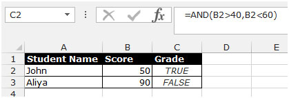
For example:Cell A1 contains student name, B1 contains 50, and we need to check if the number is more than 40 and less than 60.
- Write the formula in cell C1
- =AND(B2>40,B2<60), press Enter on the keyboard.
- The function will return True.
- If wechange the criteria to less than 40 and greater than 60, the function will return False.
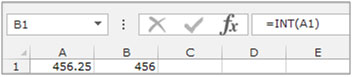
INT: — This function is used to round a number down to the nearest integer.
Syntax of “INT” function: =INT (number)
Example:Cell A1 contains the number 456.25
=INT (A1), function will return 456
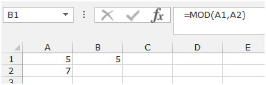
MOD: — This function is used to return the remainder after a number is divided by a divisor.
Syntax of “MOD” function: =MOD (number, divisor)
Example:Cell A1 contains the number 5, and cell A2 contains 7
=MOD (A1,A2), function will return 5
The IF function will check the logical test, the AND function will check multiple criteria, the CHAR function will provide the character as per the number, the INT function will round the number down and the Mod function will return the balance for completing the calculation in Microsoft Excel.
Let’s take an example to understand how we can change the column number to a letterin Microsoft Excel.
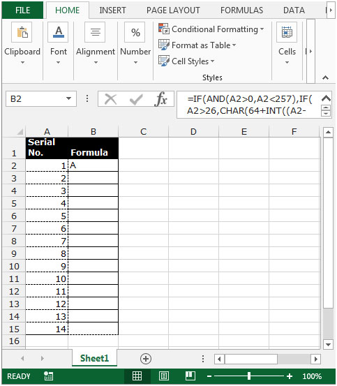
We have a serial no in column A. In column B, we need to put a formula to convert the numbers to letters.
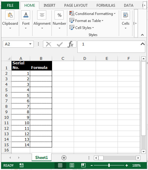
Follow the below given steps:-
- Select the cell B2 and write the formula.
- =IF(AND(A2>0,A2<257),IF(A2>26,CHAR(64+INT((A2-1)/26)),»»)&CHAR(65+MOD(A2-1,26)),»»)
- Press Enter on the keyboard.
- The function will convert the number to the letter.
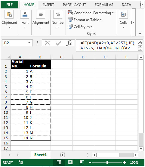
- To convert all the serial numbers into letters, copy the same formula by pressing the key Ctrl+Cand paste in the range B3:B15 by pressing the key Ctrl+Von your keyboard.
Note: This function will convert the serial numbers into letters till number 256. If you want to convert the numbers which are greater than 256, you will need to change the number in the formula.
If you had your text in CELL E1, you could use the below formula to create the number combination:
=IFERROR(INDEX(B1:B10,MATCH(MID(E1,1,1),A1:A10,0),1),"")&IFERROR(INDEX(B1:B10,MATCH(MID(E1,2,1),A1:A10,0),1),"")&IFERROR(INDEX(B1:B10,MATCH(MID(E1,3,1),A1:A10,0),1),"")&IFERROR(INDEX(B1:B10,MATCH(MID(E1,4,1),A1:A10,0),1),"")&IFERROR(INDEX(B1:B10,MATCH(MID(E1,5,1),A1:A10,0),1),"")&IFERROR(INDEX(B1:B10,MATCH(MID(E1,6,1),A1:A10,0),1),"")&IFERROR(INDEX(B1:B10,MATCH(MID(E1,7,1),A1:A10,0),1),"")&IFERROR(INDEX(B1:B10,MATCH(MID(E1,8,1),A1:A10,0),1),"")
This is basically a repetition of the below:
=IFERROR(INDEX(B1:B10,MATCH(MID(E1,1,1),A1:A10,0),1),"")
However the start part of the MID part increments:
MID(E1,1,1)
This will work to a maximum length in CELL E1 of 8 character.