Excel number value formula

Excel for Microsoft 365 Excel for Microsoft 365 for Mac Excel for the web Excel 2021 Excel 2021 for Mac Excel 2019 Excel 2019 for Mac Excel 2016 Excel 2016 for Mac Excel 2013 Excel for Mac 2011 More…Less

This article describes the formula syntax and usage of the NUMBERVALUE function in Microsoft Excel.

Description

Converts text to a number, in a locale-independent way.

Syntax

NUMBERVALUE(Text, [Decimal_separator], [Group_separator ])

The NUMBERVALUE function syntax has the following arguments.

  • Text    Required. The text to convert to a number.

  • Decimal_separator    Optional. The character used to separate the integer and fractional part of the result.

  • Group_separator    Optional. The character used to separate groupings of numbers, such as thousands from hundreds and millions from thousands.

Remarks

  • If the Decimal_separator and Group_separator arguments are not specified, separators from the current locale are used.

  • If multiple characters are used in the Decimal_separator or Group_separator arguments, only the first character is used.

  • If an empty string («») is specified as the Text argument, the result is 0.

  • Empty spaces in the Text argument are ignored, even in the middle of the argument. For example, » 3 000 » is returned as 3000.

  • If a decimal separator is used more than once in the Text argument, NUMBERVALUE returns the #VALUE! error value.

  • If the group separator occurs before the decimal separator in the Text argument , the group separator is ignored.

  • If the group separator occurs after the decimal separator in the Text argument, NUMBERVALUE returns the #VALUE! error value.

  • If any of the arguments are not valid, NUMBERVALUE returns the #VALUE! error value.

  • If the Text argument ends in one or more percent signs (%), they are used in the calculation of the result. Multiple percent signs are additive if they are used in the Text argument just as they are if they are used in a formula. For example, =NUMBERVALUE(«9%%») returns the same result (0.0009) as the formula =9%%.

Example

Copy the example data in the following table, and paste it in cell A1 of a new Excel worksheet. For formulas to show results, select them, press F2, and then press Enter. If you need to, you can adjust the column widths to see all the data.

Formula

Description

Result

=NUMBERVALUE(«2.500,27″,»,»,».»)

Returns 2,500.27. The decimal separator of the text argument in the example is specified in the second argument as a comma, and the group separator is specified in the third argument as a period.

2500.27

=NUMBERVALUE(«3.5%»)

Returns 0.035. Because no optional arguments are specified, the decimal and group separators of the current locale are used. The % symbol is not shown, although the percentage is calculated.

0.035

Top of Page

Need more help?

Date yes Add (Subtract) Days to a Date Concatenate Dates Convert Date to Number Convert Date to Text Month Name to Number Create Date Range from Dates Day Number of Year Month Name from Date First Day of Month Add (Subtract) Weeks to a Date If Functions with Dates Max Date Number of Days Between Dates Number of Days in a Month Number of Weeks Between Dates Number of Years Between Dates Split Date & Time into Separate Cells Countdown Remaining Days Insert Dates Random Date Generator Using Dynamic Ranges — Year to Date Values Add (Subtract) Years to a Date Date Formula Examples Extract Day from Date Get Day Name from Date Count Days Left in Month / Year Count Workdays Left in Month / Year Get Last Day of Month Last Business Day of Month / Year Number of Work / Business Days in Month Weekday Abbreviations Auto Populate Dates Number of Months Between Dates Quarter from a Date Years of Service Change Date Format Compare Dates Time yes Add (Subtract) Hours to Time Add (Subtract) Minutes to Time Add (Subtract) Seconds to Time Add Up time (Total Time) Time Differences Change Time Format Convert Minutes to Hours Convert Time to Decimal Convert Time to Hours Convert Time to Minutes Convert Time to Seconds Military Time Round Time to Nearest 15 Minutes Overtime Calculator Number of Hours Between Times Convert Seconds to Minutes, Hours, or Time Count Hours Worked Time Differences Time Format — Show Minutes Seconds Text yes Add Commas to Cells Get First Word from Text Capitalize First Letter Clean & Format Phone #s Remove Extra Trailing / Leading Spaces Add Spaces to Cell Assign Number Value to Text Combine Cells with Comma Combine First and Last Names Convert Text String to Date Convert Text to Number Extract Text From Cell Get Last Word Remove Unwated Characters Extract Text Before or After Character How to Split Text String by Space, Comma, & More Remove Special Characters Remove First Characters from Left Substitute Multiple Values Switch First & Last Names w/ Commas Remove Specific Text from a Cell Extract Text Between Characters (Ex. Parenthesis) Add Leading Zeros to a Number Remove Line Breaks from Text Remove all Numbers from Text Reverse Text Remove Non-Numeric Characters Remove Last Character(s) From Right Separate First and Last Names Separate Text & Numbers Round yes Round Formulas Round Price to Nearest Dollar or Cent Round to Nearest 10, 100, or 1000 Round to Nearest 5 or .5 Round Percentages Round to Significant Figures Count yes Count Blank and Non-blank Cells Count Cells Between Two Numbers Count Cells not Equal to Count if Cells are in Range Count Times Word Appears in Cell Count Words in Cell Count Specific Characters in Column Count Total Number of Characters in Column Count Cells that Equal one of two Results Count Cells that do not Contain Count Cells that Contain Specific Text Count Unique Values in Range Countif — Multiple Criteria Count Total Number of Cells in Range Count Cells with Any Text Count Total Cells in a Table Lookup yes Two Dimensional VLOOKUP VLOOKUP Simple Example Vlookup — Multiple Matches Case Sensitive Lookup Case Sensitive VLOOKUP Sum if — VLOOKUP Case Sensitive Lookup Case Sensitive VLOOKUP Find Duplicates w/ VLOOKUP or MATCH INDEX MATCH MATCH Lookup — Return Cell Address (Not Value) Lookup Last Value in Column or Row Reverse VLOOKUP (Right to Left) Risk Score Bucket with VLOOKUP Sum with a VLOOKUP Function VLOOKUP & INDIRECT VLOOKUP Concatenate VLOOKUP Contains (Partial Match) 17 Reasons Why Your XLOOKUP is Not Working Double (Nested) XLOOKUP — Dynamic Columns IFERROR (& IFNA) XLOOKUP Lookup Min / Max Value Nested VLOOKUP Top 11 Alternatives to VLOOKUP (Updated 2022!) VLOOKUP – Dynamic Column Reference VLOOKUP – Fix #N/A Error VLOOKUP – Multiple Sheets at Once VLOOKUP & HLOOKUP Combined VLOOKUP & MATCH Combined VLOOKUP Between Worksheets or Spreadsheets VLOOKUP Duplicate Values VLOOKUP Letter Grades VLOOKUP Return Multiple Columns VLOOKUP Returns 0? Return Blank Instead VLOOKUP w/o #N/A Error XLOOKUP Multiple Sheets at Once XLOOKUP Between Worksheets or Spreadsheets XLOOKUP by Date XLOOKUP Duplicate Values XLOOKUP Multiple Criteria XLOOKUP Return Multiple Columns XLOOKUP Returns 0? Return Blank Instead XLOOKUP Text XLOOKUP with IF XLOOKUP With If Statement Misc. yes Sort Multiple Columns Use Cell Value in Formula Percentage Change Between Numbers Percentage Breakdown Rank Values Add Spaces to Cell CAGR Formula Average Time Decimal Part of Number Integer Part of a Number Compare Items in a List Dealing with NA() Errors Get Worksheet Name Wildcard Characters Hyperlink to Current Folder Compound Interest Formula Percentage Increase Create Random Groups Sort with the Small and Large Functions Non-volatile Function Alternatives Decrease a Number by a Percentage Calculate Percent Variance Profit Margin Calculator Convert Column Number to Letter Get Full Address of Named Range Insert File Name Insert Path Latitute / Longitude Functions Replace Negative Values Reverse List Range Convert State Name to Abbreviation Create Dynamic Hyperlinks Custom Sort List with Formula Data Validation — Custom Formulas Dynamic Sheet Reference (INDIRECT) Reference Cell in Another Sheet or Workbook Get Cell Value by Address Get Worksheet Name Increment Cell Reference List Sheet Names List Skipped Numbers in Sequence Return Address of Max Value in Range Search by Keywords Select Every Other (or Every nth) Row Basics yes Cell Reference Basics — A1, R1C1, 3d, etc. Add Up (Sum) Entire Column or Row Into to Dynamic Array Formulas Conversions yes Convert Time Zones Convert Celsius to Fahrenheit Convert Pounds to Kilograms Convert Time to Unix Time Convert Feet to Meters Convert Centimeters to Inches Convert Kilometers to Miles Convert Inches to Feet Convert Date to Julian Format Convert Column Letter to Number Tests yes Test if a Range Contains any Text Test if any Cell in Range is Number Test if a Cell Contains a Specific Value Test if Cell Contains Any Number Test if Cell Contains Specific Number Test if Cell is Number or Text If yes Percentile If Subtotal If Sumproduct If Large If and Small If Median If Concatentate If Max If Rank If TEXTJOIN If Sum yes Sum if — Begins With / Ends With Sum if — Month or Year to Date Sum if — By Year Sum if — Blank / Non-Blank Sum if — Horizontal Sum Count / Sum If — Cell Color INDIRECT Sum Sum If — Across Multiple Sheets Sum If — By Month Sum If — Cells Not Equal To Sum If — Not Blank Sum if — Between Values Sum If — Week Number Sum Text Sum if — By Category or Group Sum if — Cell Contains Specific Text (Wildcards) Sum if — Date Rnage Sum if — Dates Equal Sum if — Day of Week Sum if — Greater Than Sum if — Less Than Average yes Average Non-Zero Values Average If — Not Blank Average — Ignore 0 Average — Ignore Errors Math yes Multiplication Table Cube Roots nth Roots Square Numbers Square Roots Calculations yes Calculate a Ratio Calculate Age KILLLLLLL Calculate Loan Payments GPA Formula Calculate VAT Tax How to Grade Formulas Find yes Find a Number in a Column / Workbook Find Most Frequent Numbers Find Smallest n Values Find nth Occurance of Character in Text Find and Extract Number from String Find Earliest or Latest Date Based on Criteria Find First Cell with Any Value Find Last Row Find Last Row with Data Find Missing Values Find Largest n Values Most Frequent Number Conditional Formatting yes Conditional Format — Dates & Times Conditional Format — Highlight Blank Cells New Functions XLOOKUP Replaces VLOOKUP, HLOOKUP, and INDEX / MATCH Logical yes AND Checks whether all conditions are met. TRUE/FALSE IF If condition is met, do something, if not, do something else. IFERROR If result is an error then do something else. NOT Changes TRUE to FALSE and FALSE to TRUE. OR Checks whether any conditions are met. TRUE/FALSE XOR Checks whether one and only one condition is met. TRUE/FALSE Lookup & Reference yes FALSE The logical value: FALSE. TRUE The logical value: TRUE. ADDRESS Returns a cell address as text. AREAS Returns the number of areas in a reference. CHOOSE Chooses a value from a list based on it’s position number. COLUMN Returns the column number of a cell reference. COLUMNS Returns the number of columns in an array. HLOOKUP Lookup a value in the first row and return a value. HYPERLINK Creates a clickable link. INDEX Returns a value based on it’s column and row numbers. INDIRECT Creates a cell reference from text. LOOKUP Looks up values either horizontally or vertically. MATCH Searches for a value in a list and returns its position. OFFSET Creates a reference offset from a starting point. ROW Returns the row number of a cell reference. ROWS Returns the number of rows in an array. TRANSPOSE Flips the oriention of a range of cells. VLOOKUP Lookup a value in the first column and return a value. Date & Time yes DATE Returns a date from year, month, and day. DATEDIF Number of days, months or years between two dates. DATEVALUE Converts a date stored as text into a valid date DAY Returns the day as a number (1-31). DAYS Returns the number of days between two dates. DAYS360 Returns days between 2 dates in a 360 day year. EDATE Returns a date, n months away from a start date. EOMONTH Returns the last day of the month, n months away date. HOUR Returns the hour as a number (0-23). MINUTE Returns the minute as a number (0-59). MONTH Returns the month as a number (1-12). NETWORKDAYS Number of working days between 2 dates. NETWORKDAYS.INTL Working days between 2 dates, custom weekends. NOW Returns the current date and time. SECOND Returns the second as a number (0-59) TIME Returns the time from a hour, minute, and second. TIMEVALUE Converts a time stored as text into a valid time. TODAY Returns the current date. WEEKDAY Returns the day of the week as a number (1-7). WEEKNUM Returns the week number in a year (1-52). WORKDAY The date n working days from a date. WORKDAY.INTL The date n working days from a date, custom weekends. YEAR Returns the year. YEARFRAC Returns the fraction of a year between 2 dates. Engineering yes CONVERT Convert number from one unit to another. Financial yes FV Calculates the future value. PV Calculates the present value. NPER Calculates the total number of payment periods. PMT Calculates the payment amount. RATE Calculates the interest Rate. NPV Calculates the net present value. IRR The internal rate of return for a set of periodic CFs. XIRR The internal rate of return for a set of non-periodic CFs. PRICE Calculates the price of a bond. YIELD Calculates the bond yield. INTRATE The interest rate of a fully invested security. Information yes CELL Returns information about a cell. ERROR.TYPE Returns a value representing the cell error. ISBLANK Test if cell is blank. TRUE/FALSE ISERR Test if cell value is an error, ignores #N/A. TRUE/FALSE ISERROR Test if cell value is an error. TRUE/FALSE ISEVEN Test if cell value is even. TRUE/FALSE ISFORMULA Test if cell is a formula. TRUE/FALSE ISLOGICAL Test if cell is logical (TRUE or FALSE). TRUE/FALSE ISNA Test if cell value is #N/A. TRUE/FALSE ISNONTEXT Test if cell is not text (blank cells are not text). TRUE/FALSE ISNUMBER Test if cell is a number. TRUE/FALSE ISODD Test if cell value is odd. TRUE/FALSE ISREF Test if cell value is a reference. TRUE/FALSE ISTEXT Test if cell is text. TRUE/FALSE N Converts a value to a number. NA Returns the error: #N/A. TYPE Returns the type of value in a cell. Math yes ABS Calculates the absolute value of a number. AGGREGATE Define and perform calculations for a database or a list. CEILING Rounds a number up, to the nearest specified multiple. COS Returns the cosine of an angle. DEGREES Converts radians to degrees. DSUM Sums database records that meet certain criteria. EVEN Rounds to the nearest even integer. EXP Calculates the exponential value for a given number. FACT Returns the factorial. FLOOR Rounds a number down, to the nearest specified multiple. GCD Returns the greatest common divisor. INT Rounds a number down to the nearest integer. LCM Returns the least common multiple. LN Returns the natural logarithm of a number. LOG Returns the logarithm of a number to a specified base. LOG10 Returns the base-10 logarithm of a number. MOD Returns the remainder after dividing. MROUND Rounds a number to a specified multiple. ODD Rounds to the nearest odd integer. PI The value of PI. POWER Calculates a number raised to a power. PRODUCT Multiplies an array of numbers. QUOTIENT Returns the integer result of division. RADIANS Converts an angle into radians. RAND Calculates a random number between 0 and 1. RANDBETWEEN Calculates a random number between two numbers. ROUND Rounds a number to a specified number of digits. ROUNDDOWN Rounds a number down (towards zero). ROUNDUP Rounds a number up (away from zero). SIGN Returns the sign of a number. SIN Returns the sine of an angle. SQRT Calculates the square root of a number. SUBTOTAL Returns a summary statistic for a series of data. SUM Adds numbers together. SUMIF Sums numbers that meet a criteria. SUMIFS Sums numbers that meet multiple criteria. SUMPRODUCT Multiplies arrays of numbers and sums the resultant array. TAN Returns the tangent of an angle. TRUNC Truncates a number to a specific number of digits. Stats yes AVERAGE Averages numbers. AVERAGEA Averages numbers. Includes text & FALSE =0, TRUE =1. AVERAGEIF Averages numbers that meet a criteria. AVERAGEIFS Averages numbers that meet multiple criteria. CORREL Calculates the correlation of two series. COUNT Counts cells that contain a number. COUNTA Count cells that are non-blank. COUNTBLANK Counts cells that are blank. COUNTIF Counts cells that meet a criteria. COUNTIFS Counts cells that meet multiple criteria. FORECAST Predict future y-values from linear trend line. FREQUENCY Counts values that fall within specified ranges. GROWTH Calculates Y values based on exponential growth. INTERCEPT Calculates the Y intercept for a best-fit line. LARGE Returns the kth largest value. LINEST Returns statistics about a trendline. MAX Returns the largest number. MEDIAN Returns the median number. MIN Returns the smallest number. MODE Returns the most common number. PERCENTILE Returns the kth percentile. PERCENTILE.INC Returns the kth percentile. Where k is inclusive. PERCENTILE.EXC Returns the kth percentile. Where k is exclusive. QUARTILE Returns the specified quartile value. QUARTILE.INC Returns the specified quartile value. Inclusive. QUARTILE.EXC Returns the specified quartile value. Exclusive. RANK Rank of a number within a series. RANK.AVG Rank of a number within a series. Averages. RANK.EQ Rank of a number within a series. Top Rank. SLOPE Calculates the slope from linear regression. SMALL Returns the kth smallest value. STDEV Calculates the standard deviation. STDEV.P Calculates the SD of an entire population. STDEV.S Calculates the SD of a sample. STDEVP Calculates the SD of an entire population TREND Calculates Y values based on a trendline. Text yes CHAR Returns a character specified by a code. CLEAN Removes all non-printable characters. CODE Returns the numeric code for a character. CONCATENATE Combines text together. DOLLAR Converts a number to text in currency format. EXACT Test if cells are exactly equal. Case-sensitive. TRUE/FALSE FIND Locates position of text within a cell.Case-sensitive. LEFT Truncates text a number of characters from the left. LEN Counts number of characters in text. LOWER Converts text to lower case. MID Extracts text from the middle of a cell. PROPER Converts text to proper case. REPLACE Replaces text based on it’s location. REPT Repeats text a number of times. RIGHT Truncates text a number of characters from the right. SEARCH Locates position of text within a cell.Not Case-sensitive. SUBSTITUTE Finds and replaces text. Case-sensitive. TEXT Converts a value into text with a specific number format. TRIM Removes all extra spaces from text. UPPER Converts text to upper case. VALUE Converts a number stored as text into a number.

Excel NUMBERVALUE функция

Иногда у вас может быть список чисел, которые импортируются на рабочий лист в текстовом формате, как показано на следующем снимке экрана. Excel не может распознать их как обычные числа. Как в таком случае преобразовать эти ячейки в нормальные числа? Фактически, функция ЧИСЛО в Excel может помочь вам быстро и легко преобразовать числа в текстовом формате в числовые значения.

номер документа значение функция 1


 Синтаксис:

Синтаксис функции ЧИСЛО в Excel:

=NUMBERVALUE (text, [decimal_separator], [group_separator])


 Аргументы:

  • text: Необходимые. Текст, который вы хотите преобразовать в обычное число.
  • decimal_separator: Необязательный. Символ, используемый в качестве десятичного разделителя в текстовом значении.
  • group_separator: Необязательный. Символ, используемый в качестве разделителя тысяч и миллионов в текстовом значении.

Заметки:

  • 1. Если десятичный_разделитель и group_separator не указаны, функция ЧИСЛО будет использовать разделители из текущего языкового стандарта.
  • 2. Если текстовая строка представляет собой пустую ячейку, результатом будет 0.
  • 3. #VALUE! будет возвращено значение ошибки:
    • 1). Если десятичный разделитель встречается в текстовой строке более одного раза;
    • 2). Если разделитель групп стоит после десятичного разделителя в текстовой строке;
  • 4. Если между текстовой строкой есть пустые пробелы, функция ЧИСЛО будет игнорировать их. Например, «1 0 0 0 0» возвращается как 10000.
  • 5. Если в десятичном разделителе или разделителе групп несколько символов, используется только первый символ.
  • 6. Функция ЧИСЛО применяется к Excel 2016, Excel 365 и более поздним версиям.

 Вернуть:

Возврат реального числа из числа хранится в виде текста.


 Примеры:

Пример 1. Базовое использование функции ЧИСЛО ЗНАЧ

Предположим, у меня есть список чисел, которые хранятся в текстовом формате, и я указываю десятичный разделитель и разделитель групп отдельно для каждого числа, как показано на следующем снимке экрана.

Чтобы преобразовать текст в формат действительных чисел, примените следующую формулу:

=NUMBERVALUE(A2, B2, C2)

Затем перетащите дескриптор заполнения вниз к ячейкам, к которым вы хотите применить эту формулу, и вы получите результат, как показано на скриншоте ниже:

Заметки:

1. В этой формуле A2 содержит ли ячейка текст, который вы хотите преобразовать, B2 является десятичным разделителем в тексте, а C2 содержит группу-разделитель.

2. Вы также можете использовать текстовые строки для замены ссылок на ячейки в приведенной выше формуле следующим образом:

=NUMBERVALUE(«12.432,56», «,», «.»)


Пример 2: функция NUMBERVALUE используется для работы с процентными значениями.

Если текст заканчивается одним или несколькими знаками процента (%), они будут использоваться при вычислении результата. Если имеется несколько знаков процента, функция ЧИСЛО будет рассматривать каждый знак и соответственно выдаст результаты. Смотрите скриншот:


 Дополнительные функции:

  • Функция Excel ВПРАВО
  • Функция RIGHT используется для возврата текста справа от текстовой строки.
  • Функция Excel PROPER
  • Функция ПРОПИСН используется, чтобы сделать первую букву каждого слова в текстовой строке заглавной, а все остальные символы — в нижнем регистре.
  • Функция ПОИСК в Excel
  • Функция ПОИСК может помочь вам найти позицию определенного символа или подстроки в заданной текстовой строке.

Лучшие инструменты для работы в офисе

Kutools for Excel — Помогает вам выделиться из толпы

Хотите быстро и качественно выполнять свою повседневную работу? Kutools for Excel предлагает 300 мощных расширенных функций (объединение книг, суммирование по цвету, разделение содержимого ячеек, преобразование даты и т. д.) и экономит для вас 80 % времени.

  • Разработан для 1500 рабочих сценариев, помогает решить 80% проблем с Excel.
  • Уменьшите количество нажатий на клавиатуру и мышь каждый день, избавьтесь от усталости глаз и рук.
  • Станьте экспертом по Excel за 3 минуты. Больше не нужно запоминать какие-либо болезненные формулы и коды VBA.
  • 30-дневная неограниченная бесплатная пробная версия. 60-дневная гарантия возврата денег. Бесплатное обновление и поддержка 2 года.

Лента Excel (с Kutools for Excel установлены)


Вкладка Office — включение чтения и редактирования с вкладками в Microsoft Office (включая Excel)

  • Одна секунда для переключения между десятками открытых документов!
  • Уменьшите количество щелчков мышью на сотни каждый день, попрощайтесь с рукой мыши.
  • Повышает вашу продуктивность на 50% при просмотре и редактировании нескольких документов.
  • Добавляет эффективные вкладки в Office (включая Excel), точно так же, как Chrome, Firefox и новый Internet Explorer.

Снимок экрана Excel (с установленной вкладкой Office)

Комментарии (0)


Оценок пока нет. Оцените первым!

The VALUE function in Excel gives the value of a text representing a number. For example, if we have a text as $5, this is a number format in a text. Therefore, using the VALUE formula on this data will give us 5. So, we can see how this function gives us the numerical value represented by a text in Excel.

Table of contents
  • Excel VALUE Function
    • Syntax
    • Examples to use VALUE Function in Excel
      • Example #1 – Convert TEXT into Number
      • Example #2 – Convert TIME of the day into a number
      • Example #3 – Mathematical Operations
      • Example #4 – Convert DATE into Number
      • Example #5 – Error in VALUE
      • Example #6 – Error in NAME
      • Example #7 – Text with NEGATIVE VALUE
      • Example #8 – Text with FRACTIONAL VALUE
    • Things to Remember
    • Recommended Articles

Syntax

The Value formula is as follows:

Value Formula

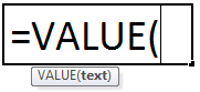
The VALUE function has only one argument, which is the required one. The VALUE formula returns a numeric value.

Where,

  • text = the text value that is to be converted into a number.

Examples to use VALUE Function in Excel

The VALUE function is a Worksheet (WS) function. As a WS function, it can be entered as a part of the formula in a worksheet cell. Refer to the examples given below to understand better.

You can download this VALUE Function Excel Template here – VALUE Function Excel Template

Example #1 – Convert TEXT into Number

VALUE function Excel Example 1

In this example, cell C2 has a VALUE formula associated with it. So, C2 is a result cell. The argument of the VALUE function is “$1,000,” the text to be converted into the number. The result is 1,000.

Example #2 – Convert the TIME of the day into a number

VALUE function Excel Example 2

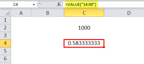
In this example, cell C4 has a VALUE formula associated with it. So, C4 is a result cell. The argument of the VALUE function is “14:00,” which is the time of the day. So, the result of converting it into a number is 0.58333.

Example #3 – Mathematical Operations

VALUE function Excel Example 3

In this example, cell C6 has a VALUE formula associated with it. So, C6 is a result cell. The argument of the VALUE function is the difference between the two values. For example, the values are “1,000” and “500”. So, the difference is 500, and the function returns the same.

Example #4 – Convert DATE into Number

VALUE Example 4

In this example, cell C8 has a VALUE formula associated with it. So, C8 is a result cell. The argument of the VALUE function is “01/12/2000,” which is the text in the date format. So, the result of converting it into the number is 36537.

Example #5 – Error in VALUE

VALUE Example 5

In this example, cell C10 has a VALUE formula associated with it. So, C10 is a result cell. Unfortunately, the argument of the VALUE function is “abc,” which is the text in an inappropriate format. Hence, we cannot process the value. As a result, #VALUE! is returned, indicating the error in value.

Example #6 – Error in NAME

VALUE Example 6

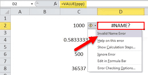
In this example, cell D2 has a VALUE formula in Excel associated with it. So, D2 is a result cell. Unfortunately, the argument of the VALUE function is ppp, which is the text in an inappropriate format, i.e., without double quotes (“). Hence, we cannot process the value.

As a result, #NAME! is returned, indicating the error is with the name provided. The same would be valid even if a valid text value is entered but not enclosed in the double quotes. E.g., VALUE (123) shall return #NAME! Error as a result.

Example #7 – Text with NEGATIVE VALUE

VALUE Example 7

In this example, cell D4 has a VALUE formula associated with it. So, D4 is a result cell. The argument of the VALUE function is “-1,” which is the text containing a negative value. As a result, the corresponding value -1 is returned by the VALUE function Excel.

Example #8 – Text with FRACTIONAL VALUE

VALUE Example 8

In this example, cell D6 has a VALUE formula in Excel associated with it. So, D6 is a result cell. The argument of the VALUE function in Excel is “0.89,” which is the text containing a fractional value. As a result, the corresponding value of 0.89 is returned by the VALUE function.

Things to Remember

  • The VALUE function converts the text into a numeric value.
  • It converts the formatted text such as date or time format into a numeric value.
  • However, Excel normally takes care of the text-to-number conversion by default. So, the VALUE function is not explicitly required.
  • It is more useful when the MS Excel data is to be made compatible with other similar spreadsheet applications.
  • It processes any numeric value less or greater than or equal to zero.
  • It processes any fractional values less or greater than or equal to zero.
  • The text entered as a parameter to be converted into the number must be enclosed within double-quotes. The #NAME! Error is returned if not done, indicating the error with the NAME entered.
  • Suppose a non-numeric text such as alphabets is entered as the parameter. In that case, the same cannot be processed by the VALUE function in Excel and returns #VALUE#VALUE! Error in Excel represents that the reference cell the user has either entered an incorrect formula or used a wrong data type (mostly numerical data). Sometimes, it is difficult to identify the kind of mistake behind this error.read more! as a result, indicating the error is with the VALUE generated.

Recommended Articles

This article has been a guide to VALUE Function in Excel. Here, we discuss the VALUE formula, how to use it, an Excel example, and a downloadable template. You may also look at these useful functions in Excel: –

  • Value Property in VBAIn VBA, the value property is usually used alongside the range method to assign a value to a range. It’s a VBA built-in expression that we can use with other functions.read more
  • Excel Shortcut Paste ValuePasting values is a common procedure that allows us to eliminate any formatting and formulas from the copied cell and paste them into the pasted cell. «Alt + E + S + V» is the shortcut key for pasting values.read more
  • NETWORKDAYS FunctionThe NETWORKDAYS function is a date and time function that determines the number of working days between two given dates  and is widely used in the fields of finance and accounting. When calculating the working days, NETWORKDAYS automatically excludes the weekend (Saturday and Sunday).read more
  • PERCENTILE Excel FunctionThe PERCENTILE function is responsible for returning the nth percentile from a supplied set of values. read more
  • Confidence Interval In ExcelConfidence Interval in excel is the range of population values that our true values lie in. read more

Функция ЗНАЧЕН преобразует текстовый аргумент в число.

Описание функции ЗНАЧЕН

Преобразует строку текста, отображающую число, в число.

Синтаксис

=ЗНАЧЕН(текст)

Аргументы

текст

Обязательный. Текст в кавычках или ссылка на ячейку, содержащую текст, который нужно преобразовать.

Замечания

  • Текст может быть в любом формате, допускаемом в Microsoft Excel для числа, даты или времени. Если текст не соответствует ни одному из этих форматов, то функция ЗНАЧЕН возвращает значение ошибки #ЗНАЧ!.
  • Обычно функцию ЗНАЧЕН не требуется использовать в формулах, поскольку необходимые преобразования значений выполняются в Microsoft Excel автоматически. Эта функция предназначена для обеспечения совместимости с другими программами электронных таблиц.

Пример

Понравилась статья? Поделить с друзьями:
  • Excel number of years
  • Excel number of selected rows
  • Excel number of rows with values
  • Excel number of days from date of
  • Excel number formatting codes