
How to Count the Number of Rows in Excel?
Here are the different ways of counting rows in Excel using the formula, rows with data, empty rows, rows with numerical values, rows with text values, and many other things related to counting the number of rows in Excel.
You can download this Count Rows Excel Template here – Count Rows Excel Template
Table of contents
- How to Count the Number of Rows in Excel?
- #1 – Excel Count Rows which has only the Data
- #2 – Count all the rows that have the data
- #3 – Count the rows that only have the numbers
- #4 – Count Rows, which only has the Blanks
- #5 – Count rows that only have text values
- #6 – Count all of the rows in the range
- Things to Remember
- Recommended Articles
#1 – Excel Count Rows which has only the Data
Firstly, we will see how to count the number of rows in Excel with the data. There could be empty rows between the data, but we often need to ignore them and find exactly how many rows contain the data in it.
- We can count the number of rows with data by selecting the range of cells in Excel. For example, take a look at the below data.

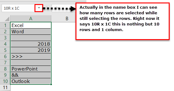
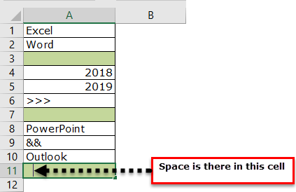
We have a total of 10 rows (border inserted area). In this 10 row, we want to count exactly how many cells have data. Since this is a small list of rows, we can easily calculate the number of rows. But when it comes to the huge database, it is impossible to count manually. So, this article will help you with this.
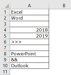
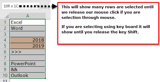
- Firstly, we must select all the rows in Excel.

- It is not telling us how many rows contain the data here. Instead, look at the Excel screen’s right-hand side bottom, i.e., a status bar.

Take a look at the red circled area. It says COUNT as 8, which means that out of 10 selected rows, 8 have data.
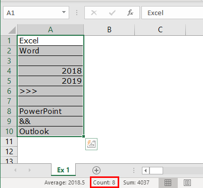
- Now, we will select one more row in the range and see what the count will be.

- We have selected 11 rows, but the count says 9, whereas we have data only in 8 rows. When we closely examine the cells, the 11th row contains a space.

Even though there is no value in the cell and it has only space Excel will be treated as the cell which contains the data.
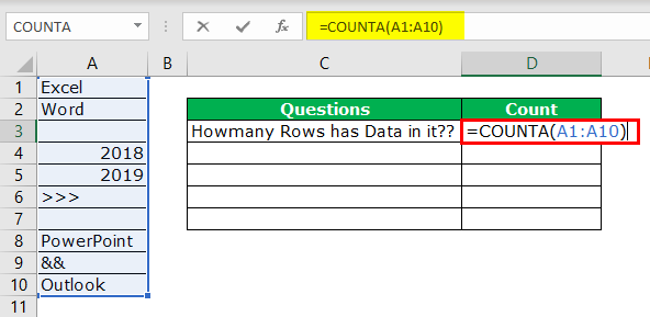
#2 – Count all the rows that have the data
We know how to check how many rows contain the data quickly. But that is not the dynamic way of counting rows that have data. Instead, we need to apply the COUNTA function to count how many rows contain the data.
We will apply the COUNTA function in the D3 cell.
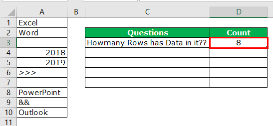
So, the total number of rows containing the data is 8 rows. Even this formula treats space as data.
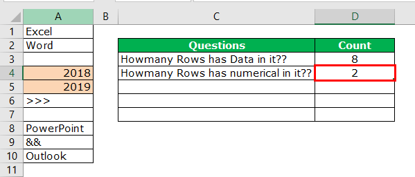
#3 – Count the rows that only have the numbers
Here we want to count how many rows contain only numerical values.
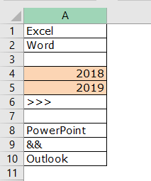
We can easily say 2 rows contain numerical values. Let us examine this by using a formula. We have a built-in formula called COUNT which counts only numerical values in the supplied range.
![]()
We will apply the COUNT function in cell B1 and select the range as A1 to A10.
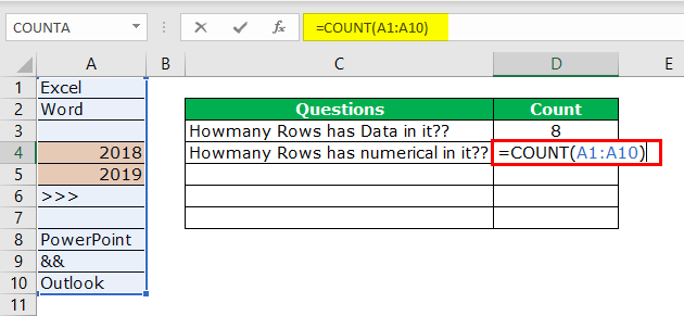
The COUNT function also says 2 as a result. So, out of 10 rows, only rows contain numerical values.
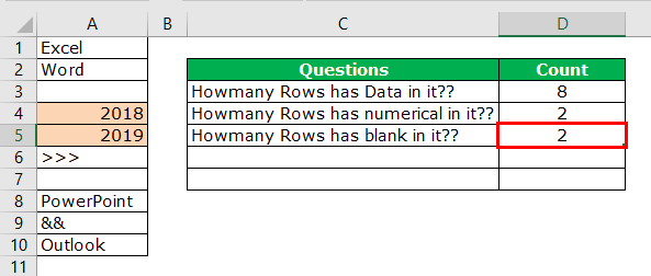
#4 – Count Rows, which only has the Blanks
We can find only blank rows by using the COUNTBLANK function in Excel.
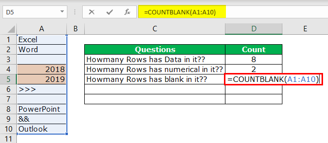
We have 2 blank rows in the selected range, which are revealed by the count blank function.
#5 – Count rows that only have text values
Remember, we do not have any straight in the COUNTTEXT function. Unlike in previous cases, we need to think differently here. We can use the COUNTIF functionThe COUNTIF function in Excel counts the number of cells within a range based on pre-defined criteria. It is used to count cells that include dates, numbers, or text. For example, COUNTIF(A1:A10,”Trump”) will count the number of cells within the range A1:A10 that contain the text “Trump”
read more with a wildcard character asterisk (*).
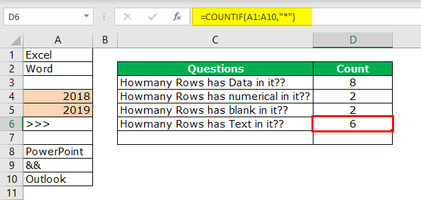
Here all the magic is done by the wildcard character asterisk (*). It matches any of the alphabets in the row and returns the result as a text value row. Even if the row contains numerical and text values, it will be treated as text value only.
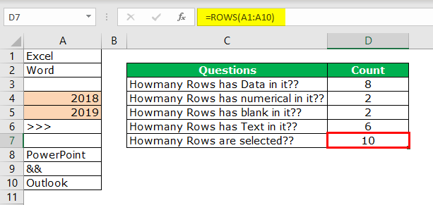
#6 – Count all of the rows in the range
Now comes the important part. How do we count how many rows we have selected? One uses the Name Box in excel, which is limited while still choosing the rows. But how do we measure then?
We have a built-in ROWS formula, which returns how many rows are selected.
Things to Remember
- Even space is treated as a value in the cell.
- If the cell contains numerical and text values, it will be treated as a text value.
- ROW may return the current row we are in, but ROWS will return how many are in the supplied range even though there is no data in the rows.
Recommended Articles
This article has been a guide to Count Rows in Excel. Here, we discuss the top 6 ways of counting rows in Excel using the formula: rows with data, empty rows, rows with numerical values, rows with text values, and many other things related to counting rows in Excel and practical examples and downloadable Excel templates. You may learn more about Excel from the following articles: –
- VBA COUNTIF
- Add Multiple Rows in Excel
- Excel Count Formula
- How to Insert Multiple Rows in Excel?
We can use an array formula to count the number of rows that contain particular values while working with excel spreadsheets. This article will provide a clear guide on how you can easily know the number of rows that have particular value. Read on to find out how to count rows that have specific values in excel.
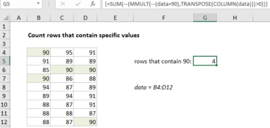 Figure 1: How to count number of rows that contain specific values
General syntax of the formula
=SUM(--(MMULT(--(criteria), TRANSPOSE(COLUMN(data)))>0))
Understanding the formula
- The above formula is fundamental when it comes to counting the number of rows that contain a particular text in excel.
- The formula is an array formula and it is based on a number if functions including MMULT, TRANSPOSE, COLUMN and SUM functions.
How the formula works
- To better understand how this formula works, we need to analyze our example in figure 1 above.
- In the figure, we have the formula in cell G5, and the formula is;
{=SUM(--(MMULT(--(B4:D12=90),TRANSPOSE, COLUMN(B4:D12)))>0))} - Notice that we have entered the formula in an array format.
- The formula has the logical criteria;
--(B4:D12=90) - This logical criteria is responsible for generating a TRUE/FALSE result for all the values in the named range of data.
- The double negative forces the TRUE/FALSE values to 1 and 0 respectively.
- Notice that the array is made up of 9 rows and 3 columns, i.e. 9×3 array. This will go to the MMULT function as array1.
- The second section of the formula is;
TRANSPOSE(COLUMN(data))
The COLUMN function is not so fundamental here. Its only work is to generate a numeric array of the right size. For the MMULT function to correctly multiple the matrix the column array1 and array2 need to be same. The COLUMN function will then return the column number in an array format. Also, the TRANSPOSE function changes the column-array format to row-array. The final array is then evaluated by the SUM function. This will count all those rows that have your particular value.
Example
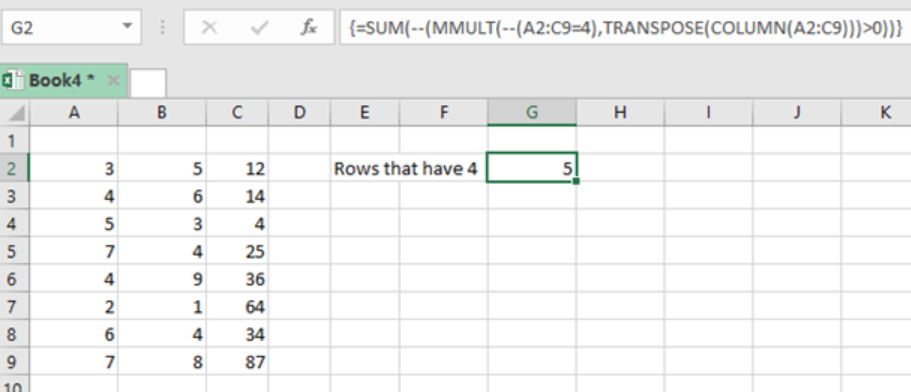 Figure 2: Example of how to count rows that contain specific value
In this example, we want to count the number of rows in that sheet that contain value 4. To do this, we proceed as follows;
Step 1: Tabulate the table with your data
Step 2: Identify the cell where you want to show the count.
Step 3: In the cell to show the count, enter the formula;
{=SUM(--(MMULT(--(A2:C9=4),TRANSPOSE(COLUMN(A2:C9)))>0))}
Step 4: Given that this is an array formula, we need to enter it in an array format. This is done by pressing the Control + Shift +Enter
Instant Connection to an Expert through our Excelchat Service
Most of the time, the problem you will need to solve will be more complex than a simple application of a formula or function. If you want to save hours of research and frustration, try our live Excelchat service! Our Excel Experts are available 24/7 to answer any Excel question you may have. We guarantee a connection within 30 seconds and a customized solution within 20 minutes.
You can use the following methods to count rows with a particular value in Excel:
Method 1: Count Rows with Any Value
=COUNTIF(B2:B11, "<>")
Method 2: Count Rows with No Value
=COUNTBLANK(B2:B11)
Method 3: Count Rows with Specific Value
=COUNTBLANK(B2:B11, "50")
The following examples show how to use each method with the following dataset in Excel:

Example 1: Count Rows with Any Value
We can use the following formula to count the number of rows with any value in column B:
=COUNTIF(B2:B11, "<>")
The following screenshot shows how to use this formula in practice:

We can see that there are 7 rows with any value in the Points column.
Example 2: Count Rows with No Value
We can use the following formula to count the number of rows with no value in column B:
=COUNTBLANK(B2:B11)
The following screenshot shows how to use this formula in practice:

We can see that there are 3 rows with no value in the Points column.
Example 3: Count Rows with Specific Value
We can use the following formula to count the number of rows with a value of “8” in column B:
=COUNTIF(B2:B11, "8")
The following screenshot shows how to use this formula in practice:

We can see that there are 3 rows with a value of “8” in the Points column.
Additional Resources
The following tutorials explain how to perform other common tasks in Excel:
How to Count Specific Words in Excel
How to Count Unique Values by Group in Excel
How to Use COUNTIF with Multiple Ranges in Excel
In this example, the goal is to count the number of rows in the data that contain the value in cell G4, which is 19. The main challenge in this problem is that the value might appear in any column, and might appear more than once in the same row. If we wanted to simply count the total number of times a value appeared in a range, we could use the COUNTIF function. But we need a more advanced formula to count rows that may contain multiple instances of the value. The explanation below reviews two options: one based on the MMULT function, and one based on the newer BYROW function.
Background study
- The double negative in Excel formulas
- Boolean operations in array formulas
- Boolean algebra in Excel
MMULT option
One option for solving this problem is the MMULT function. The MMULT function returns the matrix product of two arrays, sometimes called the «dot product». The result from MMULT is an array that contains the same number of rows as array1 and the same number of columns as array2. The MMULT function takes two arguments, array1 and array2, both of which are required. The column count of array1 must equal the row count of array2. In the example shown, the formula in G6 is:
=SUM(--(MMULT(--(data=G4),TRANSPOSE(COLUMN(data)^0))>0))
Working from the inside out, the logical criteria used in this formula is:
--(data=G4)
where data is the named range B4:D15. This expression generates a TRUE or FALSE result for every value in data, and the double negative (—) coerces the TRUE FALSE values to 1s and 0s, respectively. The result is an array of 1s and 0s like this:
{1,0,1;0,0,0;1,0,0;0,0,0;0,0,0;0,0,0;0,0,0;0,1,1;0,0,0;0,0,0;1,0,0;0,1,0}
Like the original data, this array is 12 rows by 3 columns (12 x 3) and is delivered directly to the MMULT function as array1. Array2 is derived with this snippet:
TRANSPOSE(COLUMN(data)^0)
Which returns an array of three 1s like this:
{1;1;1}
This is the tricky and fun part of this formula. The COLUMN function is used for convenience as a way to generate a numeric array of the right size. To perform matrix multiplication with MMULT, the column count in array1 (3) must equal the row count in array2 (3). COLUMN returns the 3-column array {2,3,4} which, when raised to the power of zero, becomes {1,1,1}. Next, the TRANSPOSE function transposes the 1 x 3 array into a 3 x 1 array:
TRANSPOSE({1,1,1}) // returns {1;1;1}
With both arrays in place, the MMULT function runs and returns an array with 12 rows and 1 column, {2;0;1;0;0;0;0;2;0;0;1;1}. This array contains the count per row of cells that contain 19, and we can use this data to solve the problem. Each non-zero number represents a row that contains the number 19, so we can convert non-zero values to 1s and sum up the result:
=SUM(--({2;0;1;0;0;0;0;2;0;0;1;1}>0))
We check for non-zero entries with >0 and again coerce TRUE FALSE to 1 and 0 with a double negative (—) to get a final array inside SUM:
=SUM({1;0;1;0;0;0;0;1;0;0;1;1})
In this array, 1 represents a row that contains 19 and a 0 represents a row that does not contain 19. The SUM function returns a final result of 5, the count of all rows that contain the number 19.
BYROW option
The BYROW function applies a LAMBDA function to each row in a given array and returns one result per row as a single array. The purpose of BYROW is to process data in an array or range in a «by row» fashion. For example, if BYROW is given an array with 12 rows, BYCOL will return an array with 12 results. In this example, we can use BYROW like this:
=SUM(BYROW(data,LAMBDA(row,--(SUM(--(row=G4))>0))))

The BYROW function iterates through the named range data (B4:D15) one row at a time. At each row, BYCOL evaluates and stores the result of the supplied LAMBDA function:
LAMBDA(row,--(SUM(--(row=G4))>0))
The logic here checks for values in row that are equal to G4, which results in an array of TRUE and FALSE values. The TRUE and FALSE values are coerced to 1s and 0s with the double negative (—), and the SUM function sums the result. Next, we check if the total from SUM is >0, and coerce that result to a 1 or 0. After BYROW runs, we have an array with one result per row, either a 1 or 0:
{1;0;1;0;0;0;0;1;0;0;1;1} // result from BYROW
The formula can now be simplified as follows:
=SUM({1;0;1;0;0;0;0;1;0;0;1;1}) // returns 5
In the last step, the SUM function sums the items in the array and returns a final result of 5.
Literal contains
To check for specific substrings (i.e. check to see if cells contain a specific text value) you can adjust the logic in the formulas above to use the ISNUMBER and SEARCH functions. For example, to check if a value contains «apple» you can use:
=ISNUMBER(SEARCH("apple",data))
This expression would replace data=G4 logic above like this:
=SUM(--(MMULT(--(ISNUMBER(SEARCH(G4,data))),TRANSPOSE(COLUMN(data)^0))>0))
See this example for more information on using ISNUMBER with SEARCH.
I am trying to count the number of rows in a spreadsheet which contain at least one non-blank value over a few columns: i.e.
row 1 has a text value in column A
row 2 has a text value in column B
row 3 has a text value in column C
row 4 has no values in A, B or C
The formula would equate to 3, because rows 1, 2, & 3 have a text value in at least one column. Similarly if row 1 had a text value in each column (A, B, & C) this would be counted as 1.
![]()
ashleedawg
20k8 gold badges73 silver badges104 bronze badges
asked Jul 28, 2011 at 23:39
![]()
With formulas, what you can do is:
- in a new column (say col D — cell
D2), add=COUNTA(A2:C2) - drag this formula till the end of your data (say cell
D4in our example) - add a last formula to sum it up (e.g in cell
D5):=SUM(D2:D4)
answered Jul 29, 2011 at 8:06
![]()
JMaxJMax
25.9k12 gold badges69 silver badges88 bronze badges
2
If you want a simple one liner that will do it all for you (assuming by no value you mean a blank cell):
=(ROWS(A:A) + ROWS(B:B) + ROWS(C:C)) - COUNTIF(A:C, "")
If by no value you mean the cell contains a 0
=(ROWS(A:A) + ROWS(B:B) + ROWS(C:C)) - COUNTIF(A:C, 0)
The formula works by first summing up all the rows that are in columns A, B, and C (if you need to count more rows, just increase the columns in the range. E.g. ROWS(A:A) + ROWS(B:B) + ROWS(C:C) + ROWS(D:D) + ... + ROWS(Z:Z)).
Then the formula counts the number of values in the same range that are blank (or 0 in the second example).
Last, the formula subtracts the total number of cells with no value from the total number of rows. This leaves you with the number of cells in each row that contain a value
![]()
TylerH
20.6k64 gold badges76 silver badges97 bronze badges
answered Dec 4, 2015 at 17:08
![]()
Jason McKindlyJason McKindly
4331 gold badge8 silver badges15 bronze badges
If you don’t mind VBA, here is a function that will do it for you. Your call would be something like:
=CountRows(1:10)
Function CountRows(ByVal range As range) As Long

Application.ScreenUpdating = False
Dim row As range
Dim count As Long

For Each row In range.Rows
    If (Application.WorksheetFunction.CountBlank(row)) - 256 <> 0 Then
        count = count + 1
    End If
Next

CountRows = count
Application.ScreenUpdating = True

End Function
How it works: I am exploiting the fact that there is a 256 row limit. The worksheet formula CountBlank will tell you how many cells in a row are blank. If the row has no cells with values, then it will be 256. So I just minus 256 and if it’s not 0 then I know there is a cell somewhere that has some value.
answered Jul 29, 2011 at 5:28
![]()
GaijinhunterGaijinhunter
14.5k4 gold badges50 silver badges57 bronze badges
Try this scenario:
Array = A1:C7. A1-A3 have values, B2-B6 have value and C1, C3 and C6 have values.
To get a count of the number of rows add a column D (you can hide it after formulas are set up) and in D1 put formula =If(Sum(A1:C1)>0,1,0). Copy the formula from D1 through D7 (for others searching who are not excel literate, the numbers in the sum formula will change to the row you are on and this is fine).
Now in C8 make a sum formula that adds up the D column and the answer should be 6. For visually pleasing purposes hide column D.
![]()
JMax
25.9k12 gold badges69 silver badges88 bronze badges
answered Apr 29, 2012 at 18:15
![]()
You should use the sumif function in Excel:
=SUMIF(A5:C10;"Text_to_find";C5:C10)
This function takes a range like this square A5:C10 then you have some text to find this text can be in A or B then it will add the number from the C-row.
![]()
TylerH
20.6k64 gold badges76 silver badges97 bronze badges
answered Dec 13, 2012 at 11:08
![]()
1
This is what I finally came up with, which works great!
{=SUM(IF((ISTEXT('Worksheet Name!A:A))+(ISTEXT('CCSA Associates'!E:E)),1,0))-1}
Don’t forget since it is an array to type the formula above without the «{}», and to CTRL + SHIFT + ENTER instead of just ENTER for the «{}» to appear and for it to be entered properly.
![]()
TylerH
20.6k64 gold badges76 silver badges97 bronze badges
answered Oct 29, 2015 at 15:39
![]()