Excel number and text in cell

Let’s say you need to create a grammatically correct sentence from several columns of data to prepare a mass mailing. Or, maybe you need to format numbers with text without affecting formulas that use those numbers. In Excel, there are several ways to combine text and numbers.

Use a number format to display text before or after a number in a cell

If a column that you want to sort contains both numbers and text—such as Product #15, Product #100, Product #200—it may not sort as you expect. You can format cells that contain 15, 100, and 200 so that they appear in the worksheet as Product #15, Product #100, and Product #200.

Use a custom number format to display the number with text—without changing the sorting behavior of the number. In this way, you change how the number appears without changing the value.

Follow these steps:

1. Select the cells that you want to format.

2. On the Home tab, in the Number group, click the arrow .
   

3. In the Category list, click a category such as Custom, and then click a built-in format that resembles the one that you want.

4. In the Type field, edit the number format codes to create the format that you want.

   To display both text and numbers in a cell, enclose the text characters in double quotation marks (» «), or precede the numbers with a backslash ().

   NOTE: Editing a built-in format does not remove the format.

To display	Use this code	How it works
12 as Product #12	«Product # » 0	The text enclosed in the quotation marks (including a space) is displayed before the number in the cell. In the code, «0» represents the number contained in the cell (such as 12).
12:00 as 12:00 AM EST	h:mm AM/PM «EST»	The current time is shown using the date/time format h:mm AM/PM, and the text «EST» is displayed after the time.
-12 as $-12.00 Shortage and 12 as $12.00 Surplus	$0.00 «Surplus»;$-0.00 «Shortage»	The value is shown using a currency format. In addition, if the cell contains a positive value (or 0), «Surplus» is displayed after the value. If the cell contains a negative value, «Shortage» is displayed instead.

Combine text and numbers from different cells into the same cell by using a formula

When you do combine numbers and text in a cell, the numbers become text and no longer function as numeric values. This means that you can no longer perform any math operations on them.

To combine numbers, use the CONCATENATE or CONCAT, TEXT or TEXTJOIN functions, and the ampersand (&) operator.
 

Notes: 

• In Excel 2016, Excel Mobile, and Excel for the web, CONCATENATE has been replaced with the CONCAT function. Although the CONCATENATE function is still available for backward compatibility, you should consider using CONCAT, because CONCATENATE may not be available in future versions of Excel.

• TEXTJOIN combines the text from multiple ranges and/or strings, and includes a delimiter you specify between each text value that will be combined. If the delimiter is an empty text string, this function will effectively concatenate the ranges. TEXTJOIN is not available in Excel 2013 and previous versions.

Examples

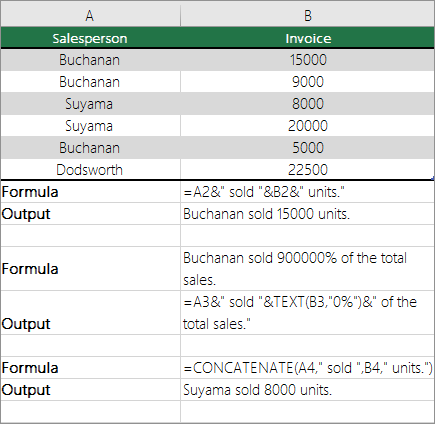
See various examples in the figure below.

Look closely at the use of the TEXT function in the second example in the figure. When you join a number to a string of text by using the concatenation operator, use the TEXT function to control the way the number is shown. The formula uses the underlying value from the referenced cell (.4 in this example) — not the formatted value you see in the cell (40%). You use the TEXT function to restore the number formatting.

Need more help?

You can always ask an expert in the Excel Tech Community or get support in the Answers community.

See Also

• CONCATENATE function

• CONCAT function

• TEXT function

• TEXTJOIN function

Combining Text and Numbers from Separate Cells

We begin with a small table that contains names (text) in column A and amounts (numbers) in column B.

Our goal is to have the name and amount for each row of the table displayed in a single cell (column C).

This needs to be done dynamically so that a change in either the name or amount will trigger an update in the combined version in column C.

This can be accomplished with a CONCATENATE function.

CONCATENATE is a big, fancy word for “join things together”.

Excel has a dedicated CONCATENATE function, but most users will opt to use the simplified version of CONCATENATE… the ampersand (&) symbol.

For example, we begin in cell C2 and write the following formula:

=A2 & B2

Pressing ENTER to commit the formula results in the following:

This is the purest form of concatenation; everything is just smashed together.  It works, but it’s not visually appealing.

Concatenation is not limited to existing content.  We can inject new content into the formula to enhance the results.  In our case, we’ll inject a ‘space’ to provide visual padding between the name and the amount.

The ‘space’ needs to be surrounded by double-quotes.  Any injected text needs to be surrounded by double-quotes.

=A2 & " " & B2

The updated formula’s result is a bit easier to read.

Think of the ampersand character as the word “and”.  “Display the name in cell A2 and a space and the number in cell B2.”

You can place anything you wish between the two double-quotes, like a dash, slash, or any other character.

Returning to using a ‘space’, we fill the formula down to the remaining rows to reveal the following:

Formatting the Numbers in the Result

If we need to represent the numbers in the result as money (we’ll use U.S. Dollars in our example) we can’t just click the dollar sign button on the ribbon.  The formatting codes for Currency Style are rendered inert with the presence of the concatenated text.

But not to worry; we have a solution.

We can apply number formatting to the result via the TEXT function.

The Excel TEXT function has the following syntax:

=TEXT(value, format_text)

• value – This can be a static value, a reference to a cell that contains a value, or a formula that returns a value.
• format_text – This is the formatting code(s) that determine the way numbers are presented.

For our numbers, we want to display a dollar sign and a comma for every three place values.  We also want to show zero if the number is zero.

Our codes for this are:

“$#,##0”

The formatting codes are always placed within a set of double-quotes.

Our formula would be updated as follows:

=A2 & " " & TEXT(B2, "$#,##0")

Committing our new formula to all rows of the tale gives us a much more appealing result.

As the values in column B change, the TEXT functions in column C will apply the appropriate number formatting.

For more information on the formatting codes and uses in the TEXT function, visit the following link.

Microsoft Excel’s TEXT Function

PRO TIP:

If you are unsure what formatting codes to use, an easy way to figure it out is to do the following:

1. Select a cell with the number you want to format (ex: cell B2) and press F1 to open the number formatting dialog box.
2. Select the category (on the left) then the desired formatting (on the right).

1. Select the “Custom” category (on the left) to reveal the underlying codes needed to support the selection from Step 2.

By applying different formatting options and examining the underlying codes, you will likely figure out many of the symbol’s purposes.

Using Aggregation Functions Inside a Formatting Function

Because the first argument in the TEXT function can be a formula, we can embed an aggregation function, like SUM, into the formula to produce a formatted aggregation.

="Base: " & TEXT(SUM(B2:B5), "$#,##0")

The SUM function provides the aggregation which is then passed off to the TEXT function that applies the formatting codes.

The final touch is to concatenate the text string “Base: ” to the front of the formatted number.

We can write a similar formula for the bonus column.

="Bonus: " & TEXT(SUM(B2:B5), "$#,##0")

“What if we want to add the ‘Base” and ‘Bonus’ results?”

If we write a SUM function that attempts to aggregate the results of the previous two formulas, we end up with a less than desirable result.

This occurs because we have embedded text in the same cell as the result of the SUM function.

Separating the Formatting from the Aggregation

We can overcome the previous issue by concatenating the desired text in a Custom Number Format to produce the same result.

This allows you to place a simple aggregation function, like SUM, in a cell without any other modifiers.

We can then select the cell containing the above formula, press F1 to open the Format Cells dialog box and apply the following custom number format.

"Base: "$#,##0

We can apply a similar formatting code sequence to the bonus columns total in cell C6.

"Bonus: "$#,##0

Adding the two SUM results now works perfectly.

NOTE: I applied the following Custom Number Format to the result to spice it up like the other aggregations.

"Total: "$#,##0

Practice Workbook

Feel free to Download the Workbook HERE.

Please Note:
This article is written for users of the following Microsoft Excel versions: 97, 2000, 2002, and 2003. If you are using a later version (Excel 2007 or later), this tip may not work for you. For a version of this tip written specifically for later versions of Excel, click here: Combining Numbers and Text in a Cell.

Many times I want a description for my data. One approach is to put the description—a simple text string—near the cell containing the data that needs describing. For instance, a numeric value could go in cell B3, and the unit description in cell C3, which read together may be something like «3.27 miles.»

Another approach is to put the description text and the numeric value together. Creating text strings easily accomplishes this feat. Here’s a very simple example that displays «1 + 1 is 2.»

="1 + 1 is " & 1+1

The quotation marks are important. By making the text string part of a formula, you can combine the description and the value within one cell.

The disadvantage of this approach is formatting the value takes more effort; since the result is a text string, numeric cell formatting does not apply. For example, consider the above formula and the need to display two decimal places. One might naturally display the Format Cell dialog box and then choose a Number format that has two decimal places, but the results would not change. (Remember, the result of the formula is text, not a number.)

To affect the value formatting, use the TEXT function. To force the above results to display the value to two decimal places, use the following formula.

="1 + 1 is " & TEXT(1+1, "0.00")

The different formats you can use with the TEXT function have been covered in other issues of ExcelTips, and you can also find more info in Excel’s Help system. Here’s an example that displays «Today is » along with today’s date. Enter the following formula in some cell:

="Today is " & TEXT(NOW(),"dddd, mmm dd, yyyy") 

Again, the quotation marks are important, as you are constructing a text string.

Author Bio

With more than 50 non-fiction books and numerous magazine articles to his credit, Allen Wyatt is an internationally recognized author. He is president of Sharon Parq Associates, a computer and publishing services company. Learn more about Allen…

Sometimes you may have the text and numeric data in the same cell, and you may have a need to separate the text portion and the number portion in different cells.

While there is no inbuilt method to do this specifically, there are some Excel features and formulas you can use to get this done.

In this tutorial, I will show you 4 simple and easy ways to separate text and numbers in Excel.

Let’s get to it!

Separate Text and Numbers Using Flash Fill

Below I have the employee data in column A, where the first few alphabets indicate the department of the employee and the numbers after it indicates the employee number.

From this data, I want to separate the text part and the number part and get these into two separate columns (columns B and C).

The first method that I want to show you to separate text and numbers in Excel is by using Flash Fill.

Flash Fill (introduced in Excel 2013) works by identifying patterns based on user input.

So if I manually enter the expected result in column B, Flash Fill will try and decipher the pattern and give me the result for all the cells in that column.

Below are the steps to separate the text part from the cell and get it in column B:

1. Select cell B2
2. Manually enter the expected result in cell B2, which would be MKT

1. With cell B2 selected, place the cursor at the bottom right part of the selection. You’ll notice that the cursor changes into a plus icon (this is called Fill Handle)

1.  Hold the left mouse/trackpad key and drag the Fill Handle to fill the cells. Don’t worry if the cells are filled with the same text
2. Click on the Auto Fill Options icon and then select the ‘Flash Fill’ option

The above steps would extract the text part from the cells in column A and give you the result in column B.

Note that in some cases, Flash Fill may not be able to identify the right pattern. In such cases, it would be best to enter the expected result in two or three cells, use the Fill Handle to fill the entire column, and then use Flash Fill on this data.

You can follow the same process to extract the numbers in column C. All you need to do is enter the expected result in cell C2 (step 2 in the process laid out above)

Note that the result you get from Flash Fill is static and would not update in case you change the original data in column A. If you want the result to be dynamic, you can use the formula method covered next.

Separate Text and Numbers Using Formula

Below I have the employee data in column A and I want to use a formula to extract only the text part and put it in column B and extract the number part and put it in column C.

Since the data is not consistent (i.e., the alphabets in the department code and the numbers in the employee number are not of the consistent length), I cannot use the LEFT or RIGHT function to extract only the text portion or only the number portion.

Below is the formula that will extract only the text portion from the left:

=LEFT(A2,MIN(IFERROR(FIND({0,1,2,3,4,5,6,7,8,9},A2),""))-1)

And below is the formula that will extract all the numbers from the right:

=MID(A2,MIN(IFERROR(FIND({0,1,2,3,4,5,6,7,8,9},A2),"")),100)

How does this formula work?

Let me first explain the formula that we use to separate the text part on the left.

=LEFT(A2,MIN(IFERROR(FIND({0,1,2,3,4,5,6,7,8,9},A2),””))-1)

The FIND part in the formula finds the position of digits 0 to 9 in cell A2. In case it finds that digit in cell A2, it returns the position of that digit, and in case it is not able to find that digit, then it returns the value error (#VALUE!)

For cell A2, it gives a result as shown below:

{#VALUE!,4,#VALUE!,#VALUE!,#VALUE!,6,#VALUE!,5,#VALUE!,#VALUE!}

• For 0, it returns #VALUE! as it cannot find this digit in cell A2
• For 1, it returns 4 as that is the position of the first occurrence of 1 in cell A2
• and so on…

This FIND formula is then wrapped inside the IFERROR function, which removes all the value errors but leaves the numbers.

The result of it looks like as shown below:

{“”,4,””,””,””,6,””,5,””,””}

The MIN function then goes through the above result and gives us the minimum value from the results. Since each number in the array represents the position of that corresponding number, the minimum value tells us where the numerical value starts in the cell.

Now that we know where the numerical values start, I have used the LEFT function to extract everything before this position (which would be all the text in the cell).

Similarly, you can use the same formula with a minor tweak to extract all the numbers after the text. To extract the numbers, where we know the starting position of the first digit, use the MID function to extract everything starting from that position.

And what if the situation is reversed – where we have the numbers first and the text later and we want to separate the numbers and text?

You can still use the same logic with one minor change – instead of finding the minimum value that gives us the position of the 1st digit in the cell, you need to use the MAX function To find the position of the last digit in this cell. Once you have it, you can again use the LEFT function or the MID function to separate the numbers and text.

Separate Text and Numbers Using VBA (Custom Function)

While you can use the formulas shown above to separate the text and numbers in a cell and extract these into different cells – if this is something you need to do quite often, you also have the option to create your own custom function using VBA.

The benefit of creating your own function would be that it would be a lot easier to use (with just one function that takes only one argument).

You can also save this custom function VBA code into the Personal Macro Workbook so that it would be available in all your Excel workbooks.

Below the VBA code that could create a function ‘GetNumber’ that would take the cell reference as the input argument, extract all the numbers in the cell, and give it as the result.

'Code created by Sumit Bansal from https://trumpexcel.com
'This code will create a function that can separate numbers from a cell
Function GetNumber(CellRef As String)
Dim StringLength As Integer
StringLength = Len(CellRef)
For i = 1 To StringLength
If IsNumeric(Mid(CellRef, i, 1)) Then Result = Result & Mid(CellRef, i, 1)
Next i
GetNumber = Result
End Function

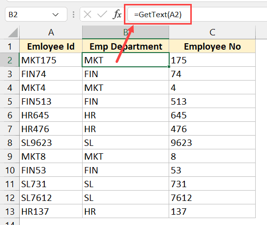
And below the VBA code that would create another function ‘GetText’ that would take the cell reference as the input argument and give you all the text from that cell

'Code created by Sumit Bansal from https://trumpexcel.com
''This code will create a function that can separate text from a cell
Function GetText(CellRef As String)
Dim StringLength As Integer
StringLength = Len(CellRef)
For i = 1 To StringLength
If Not (IsNumeric(Mid(CellRef, i, 1))) Then Result = Result & Mid(CellRef, i, 1)
Next i
GetText = Result
End Function

Below are the steps to add this code to your excel workbook so that this function becomes available for you to use in the worksheet:

1. Click the Developer tab in the ribbon
2. Click on the Visual Basic icon

1. In the Visual Basic editor that opens up, you would see the Project Explorer on the left. This would have the workbook and the worksheet names of your current Excel workbook. If you don’t see this, click on the View option in the menu and then click on Project Explorer

1. Select any of the sheet names (or any object) for the workbook in which you want to add this function
2. Click on the Insert option in the top toolbar and then click on Module. This will insert a new module for that workbook

1. Double click on the module icon in ‘Project Explorer’. This will open the module code window.

1. Copy and paste the above custom function code into the module code window

1. Close the VB Editor

With the above steps, we have added the custom function code to the Excel workbook.

Now you can use the functions =GETNUMBER or =GETTEXT just like any other worksheet function.

Note – Once you have the macro code in the module code window, you need to save the file as a Macro Enabled file (with the .xlsm extension instead of the .xlsx extension)

If you often have a need to separate text numbers from cells in Excel, it would be more efficient if you copy these VBA codes for creating these custom functions, and save these in your Personal Macro Workbook.

You can learn how to create and use Personal Macro Workbook in this tutorial I created earlier.

Once you have these functions in the Personal Macro Workbook, you would be able to use these on any Excel workbook on your system.

One important thing to remember when using functions that are stored in Personal Macro Workbook – you need to prefix the function name with =PERSONAL.XLSB!. For example, if I want to use the function GETNUMBER in a workbook in Excel, and I have saved the code for it in the postal macro workbook, I will have to use =PERSONAL.XLSB!GETNUMBER(A2)

Separate Text and Numbers Using Power Query

Power Query is slowly becoming my favorite feature in Excel.

If you’re already using Power Query as a part of your workflow, and you have a data set where you want to separate the text and numbers into separate columns, Power Query will do it in a few clicks.

When you have your data in Excel and you want to use Power Query to transform that data, one prerequisite is to convert that data into an Excel Table (or a named range).

Below I have an Excel Table that contains the data where I want to separate the text and number portions into separate columns.

Here are the steps to do this:

1. Select any cell in the Excel Table
2. Click the Data tab in the ribbon

1. In the Get and Transform group, click on the ‘From Table/Range’

1. In the Power Query editor that opens up, select the column from which you want to separate the numbers and text
2. Click the Transform tab in the Power Query ribbon

1. Click on the Split Column option

1. Click on ‘By Non Digit to Digit’ option.

1. You’ll see that the column has been split into two columns where one has only the text and the other only has the numbers

1. [Optional] Change the column names if you want
2. Click the Home tab and then click on Close and Load. This will insert a new sheet and give us the output as an Excel Table.

The above steps would take the data from the Excel Table we originally had, use Power Query to split the column and separate the text and the number parts into two separate columns, and then give us back the output in a new sheet in the same workbook.

Note that we used the option ‘By Non-Digit to Digit’ option in step 7, which means that every time there is a change from a non-digit character to a digit, a split would be made. If you have a dataset where the numbers are first followed by text, you can use the ‘By Digit to Non-Digit’ option

Now let me tell you the best part about this method. Your original Excel Table (which is the data source) is connected to the output Excel Table.

So if you make any changes in your original data, you don’t need to repeat the entire process. You can simply go to any cell in the output Excel Table, right click and then click on Refresh.

Power query would run in the back end, check the entire original data source, do all the transformations that we did in the steps above, and update your output result data.

This is where Power Query really shines. If there is a set of transformations that you often need to do on a data set, you can use Power Query to do that transformation once and set the process. Excel would create a connection between the original data source and the resulting output data and remember all the steps you had taken to transform this data.

Now, if you get a new data set you can simply put it in the place of your original data and refresh the query, and you will get the result in a few seconds. Alternatively, you can simply change the source in Power Query from the existing Excel table to some other Excel Table (in same or different workbook).

So these are four simple ways you can use to separate numbers and text in Excel. if this is a once-in-a-while activity, you’re better off using Flash Fill or the formula method.

And in case this is something you need to do quite often, then I would suggest you consider the VBA method where we created a custom function or the Power Query method.

I hope you found this Excel tutorial useful.

Other Excel tutorials you may also like:

• Separate First and Last Name in Excel (Split Names Using Formulas)
• How to Convert Numbers to Text in Excel
• Convert Text to Numbers in Excel – A Step By Step Tutorial
• How to Compare Text in Excel
• How to Quickly Combine Cells in Excel
• How to Combine First and Last Name in Excel
• How to Extract the First Word from a Text String in Excel (3 Easy Ways)
• Extract Numbers from a String in Excel (Using Formulas or VBA)
• How to Extract a Substring in Excel (Using TEXT Formulas)

In all versions of Excel, you can use a simple formula, with the & operator, to combine values from different cells. If you want the numbers formatted a certain way, use the TEXT function to set that up.

Video: Combine Text and Numbers

First, this video shows a simple formula to combine text and numbers in Excel. Then, see how to use the Excel TEXT function, to format the numbers in the formula.

You can type the formatting information inside the TEXT function. Or, put the formatting string in a different cell, and refer to that cell in the TEXT function.

To follow along, get the sample file on my Contextures site – How to Combine Cells

TEXTJOIN – Excel 365

If you’re using Excel 365, there’s a new TEXTJOIN function. It makes it easy to combine values from multiple cells.

This short video shows a couple of TEXTJOIN examples. First, see a simple formula to combine weekday names. Next, use the TEXT function inside TEXTJOIN, create formatted dates. There are written steps, and more examples, on my Contextures website.

Simple Formula

Even if you don’t have the new TEXTJOIN function, it’s easy combine values from multiple cells, using a simple formula. Just use the & (ampersand) operator, to join values together.

In this example:

• There’s text in cell A2, with a space character at the end.
• There’s an unformatted number in cell B2.

This formula, in cell C2, combines the text and number:

=A2 & B2

Or, if the text does not have a space character at the end, add one in the formula

=A2 & " " & B2

Format Numbers with TEXT Function

To join text with formatted numbers, use the TEXT function in the formula.

In this example:

• There’s text in cell A2, with a space character at the end.
• There’s a formatted date in cell B2.

This formula, in cell C2, combines the text and date, with formatting:

=A2 & TEXT(B2,"d-mmm")

Number Format Information

Instead of typing the number format inside the TEXT function, you could type those formats in another column, or on a different worksheet.

Then, in the TEXT function, refer to the cell with the required format.

For example, I’ve made a formatting list with named cells. Now, I can use those names in the TEXT function.

• FmtDMY    d-mmm-yyyy
• FmtCurr    $#,##0
• FmtFrac    # ?/?

In this example, the formula in C2 uses the d-mmm-yyyy format, from the cell named FmtDMY:

=A2 & TEXT(B2,FmtDMY)

The other named formats are used in cells C5 and C8.

Currency – cell C5

=A5 & TEXT(B5,FmtCurr)

Fraction – cell C8

=A8 & TEXT(B8,FmtFrac)

Get the Workbook

To see more examples of combining text and numbers, and to get the sample workbook, go to the Combine Cells page on my Contextures site.

The zipped file is in xlsx format, and does not contain any macros.

________________________________

Combine Text and Formatted Numbers in Excel

________________________________