
So, there are times when you would like to know that a value is in a list or not. We have done this using VLOOKUP. But we can do the same thing using COUNTIF function too. So in this article, we will learn how to check if a values is in a list or not using various ways.
Check If Value In Range Using COUNTIF Function
So as we know, using COUNTIF function in excel we can know how many times a specific value occurs in a range. So if we count for a specific value in a range and its greater than zero, it would mean that it is in the range. Isn’t it?
Generic Formula
=COUNTIF(range,value)>0
Range: The range in which you want to check if the value exist in range or not.
Value: The value that you want to check in the range.
Let’s see an example:
Excel Find Value is in Range Example
For this example, we have below sample data. We need a check-in the cell D2, if the given item in C2 exists in range A2:A9 or say item list. If it’s there then, print TRUE else FALSE.
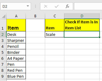
Write this formula in cell D2:
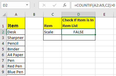
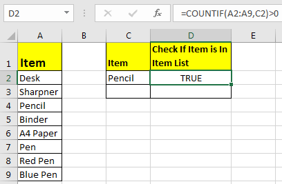
Since C2 contains “scale” and it’s not in the item list, it shows FALSE. Exactly as we wanted. Now if you replace “scale” with “Pencil” in the formula above, it’ll show TRUE.
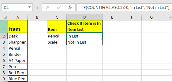
Now, this TRUE and FALSE looks very back and white. How about customizing the output. I mean, how about we show, “found” or “not found” when value is in list and when it is not respectively.
Since this test gives us TRUE and FALSE, we can use it with IF function of excel.
Write this formula:
=IF(COUNTIF(A2:A9,C2)>0,»in List»,»Not in List»)
You will have this as your output.
What If you remove “>0” from this if formula?
=IF(COUNTIF(A2:A9,C2),»in List»,»Not in List»)
It will work fine. You will have same result as above. Why? Because IF function in excel treats any value greater than 0 as TRUE.
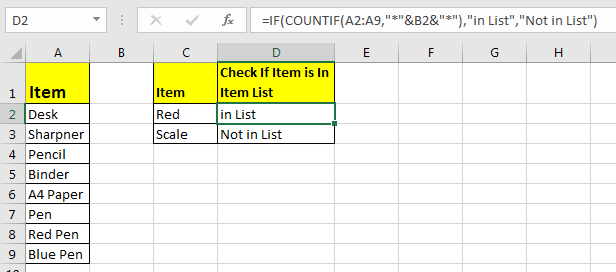
How to check if a value is in Range with Wild Card Operators
Sometimes you would want to know if there is any match of your item in the list or not. I mean when you don’t want an exact match but any match.
For example, if in the above-given list, you want to check if there is anything with “red”. To do so, write this formula.
=IF(COUNTIF(A2:A9,»*red*»),»in List»,»Not in List»)
This will return a TRUE since we have “red pen” in our list. If you replace red with pink it will return FALSE. Try it.
Now here I have hardcoded the value in list but if your value is in a cell, say in our favourite cell B2 then write this formula.
IF(COUNTIF(A2:A9,»*»&B2&»*»),»in List»,»Not in List»)
There’s one more way to do the same. We can use the MATCH function in excel to check if the column contains a value. Let’s see how.
Find if a Value is in a List Using MATCH Function
So as we all know that MATCH function in excel returns the index of a value if found, else returns #N/A error. So we can use the ISNUMBER to check if the function returns a number.
If it returns a number ISNUMBER will show TRUE, which means it’s found else FALSE, and you know what that means.
Write this formula in cell C2:
=ISNUMBER(MATCH(C2,A2:A9,0))
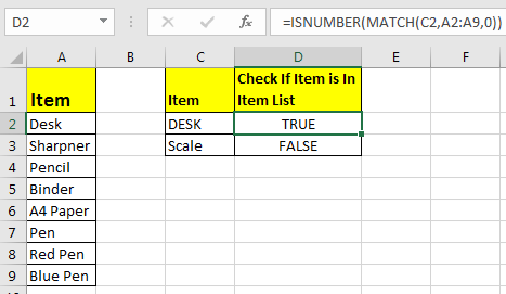
The MATCH function looks for an exact match of value in cell C2 in range A2:A9. Since DESK is on the list, it shows a TRUE value and FALSE for SCALE.
So yeah, these are the ways, using which you can find if a value is in the list or not and then take action on them as you like using IF function. I explained how to find value in a range in the best way possible. Let me know if you have any thoughts. The comments section is all yours.
Related Articles:
How to Check If Cell Contains Specific Text in Excel
How to Check A list of Texts In String in Excel
How to take the Average Difference between lists in Excel
How to Get Every Nth Value From A list in Excel
Popular Articles:
50 Excel Shortcuts to Increase Your Productivity
How to use the VLOOKUP Function in Excel
How to use the COUNTIF function in Excel
How to use the SUMIF Function in Excel
I’ve got a range (A3:A10) that contains names, and I’d like to check if the contents of another cell (D1) matches one of the names in my list.
I’ve named the range A3:A10 ‘some_names’, and I’d like an excel formula that will give me True/False or 1/0 depending on the contents.
asked May 29, 2013 at 20:43
![]()
joseph.hainlinejoseph.hainline
2,0523 gold badges16 silver badges16 bronze badges
=COUNTIF(some_names,D1)
should work (1 if the name is present — more if more than one instance).
answered May 29, 2013 at 20:47
![]()
1
My preferred answer (modified from Ian’s) is:
=COUNTIF(some_names,D1)>0
which returns TRUE if D1 is found in the range some_names at least once, or FALSE otherwise.
(COUNTIF returns an integer of how many times the criterion is found in the range)
![]()
pnuts
6,0623 gold badges27 silver badges41 bronze badges
answered Jun 6, 2013 at 20:40
![]()
joseph.hainlinejoseph.hainline
2,0523 gold badges16 silver badges16 bronze badges
0
I know the OP specifically stated that the list came from a range of cells, but others might stumble upon this while looking for a specific range of values.
You can also look up on specific values, rather than a range using the MATCH function. This will give you the number where this matches (in this case, the second spot, so 2). It will return #N/A if there is no match.
=MATCH(4,{2,4,6,8},0)
You could also replace the first four with a cell. Put a 4 in cell A1 and type this into any other cell.
=MATCH(A1,{2,4,6,8},0)
![]()
answered Nov 10, 2014 at 22:57
![]()
RPh_CoderRPh_Coder
4784 silver badges4 bronze badges
6
If you want to turn the countif into some other output (like boolean) you could also do:
=IF(COUNTIF(some_names,D1)>0, TRUE, FALSE)
Enjoy!
answered May 29, 2013 at 21:09
![]()
1
For variety you can use MATCH, e.g.
=ISNUMBER(MATCH(D1,A3:A10,0))
answered May 29, 2013 at 23:28
![]()
barry houdinibarry houdini
10.8k1 gold badge20 silver badges25 bronze badges
there is a nifty little trick returning Boolean in case range some_names could be specified explicitly such in "purple","red","blue","green","orange":
=OR("Red"={"purple","red","blue","green","orange"})
Note this is NOT an array formula
answered Jul 11, 2018 at 22:06
![]()
gregVgregV
2042 silver badges4 bronze badges
1
You can nest --([range]=[cell]) in an IF, SUMIFS, or COUNTIFS argument. For example, IF(--($N$2:$N$23=D2),"in the list!","not in the list"). I believe this might use memory more efficiently.
Alternatively, you can wrap an ISERROR around a VLOOKUP, all wrapped around an IF statement. Like, IF( ISERROR ( VLOOKUP() ) , "not in the list" , "in the list!" ).
answered Dec 5, 2013 at 19:33
![]()
0
In situations like this, I only want to be alerted to possible errors, so I would solve the situation this way …
=if(countif(some_names,D1)>0,"","MISSING")
Then I’d copy this formula from E1 to E100. If a value in the D column is not in the list, I’ll get the message MISSING but if the value exists, I get an empty cell. That makes the missing values stand out much more.
![]()
answered Aug 24, 2013 at 11:59
![]()
0
Array Formula version (enter with Ctrl + Shift + Enter):
=OR(A3:A10=D1)
answered Dec 8, 2016 at 12:38
![]()
SlaiSlai
1195 bronze badges
1
Summary
Note: Excel has a built-in data validation rules for dropdown lists. This page explains how to create a custom validation rule when you want to *prevent* a user from entering a value in a list.
To allow only values that do not exist in a list, you can use data validation with a custom formula based on the COUNTIF function. In the example shown, the data validation applied to B5:B9 is:
=COUNTIF(list,B5)=0
where «list» is the named range D5:D7.
Generic formula
Explanation
Data validation rules are triggered when a user adds or changes a cell value.
In this case, the COUNTIF function is part of an expression that returns TRUE when a value does not exist in a defined list. The COUNTIF function simply counts occurrences of the value in the list. As long as the count is zero, the entry will pass validation. If the count is not zero (i.e. the user entered a value from the list) validation will fail.
Note: Cell references in data validation formulas are relative to the upper left cell in the range selected when the validation rule is defined, in this case B5.

Author![]()
Dave Bruns
Hi — I’m Dave Bruns, and I run Exceljet with my wife, Lisa. Our goal is to help you work faster in Excel. We create short videos, and clear examples of formulas, functions, pivot tables, conditional formatting, and charts.
There are hundreds and hundreds of Excel sites out there. I’ve been to many and most are an exercise in frustration. Found yours today and wanted to let you know that it might be the simplest and easiest site that will get me where I want to go.
Get Training
Quick, clean, and to the point training
Learn Excel with high quality video training. Our videos are quick, clean, and to the point, so you can learn Excel in less time, and easily review key topics when needed. Each video comes with its own practice worksheet.
View Paid Training & Bundles
Help us improve Exceljet
I’m trying to count rows when values of a column are equal to a specific value AND, at the same time, a value of an another column is not in a list.
For example imagine the following table :
A  B       C
ID COUNTRY COLOR
1  GER     blue
2  GER     green
3  FRA     blue
4  USA     red
5  GER     red
6  FRA     blue
7  GER     green
8  FRA     red
9  GER     gold
I Would like to count each rows where:
- COUNTRY = GER
- COLOR is not equal to red or blue
I tried the following formula:
=SUM(COUNTIFS(B:B;"GER;C:C{"<>red";"<>blue"}))
I was expecting 3 because I would like to count rows where the country is «GER» and color is everything except red and blue (Line 2, 7 and 9).
BUT output is 8.
This is surely because Excel detects 4 lines where the country is GER and color not red (1,2,7,9) + 4 lines GER and color not blue (2,5,7,9).
I know it is not complicated, but I can’t figure it out.
Maybe one of you could give me a hint on how deals with my problem? Thanks a lot.
Содержание
- 0.1 Простейший способ
- 0.1.1 Excel
- 0.1.2 Calc
- 0.2 Простейший способ
- 0.2.1 Excel
- 0.2.2 Calc
- 0.3 Мудрейший способ
- 0.3.1 Excel
- 0.3.2 Calc
- 0.3.3 Кстати
- 1 , но можно и «неформально» обрамить его тэгом — и покажи мне разницу…«, но имеет место бывать. Выделите ячейки с данными, которые должны попасть в выпадающий список (например, наименованиями товаров). Выберите в меню Вставка — Имя — Присвоить (Insert — Name — Define) и введите имя (можно любое, но обязательно без пробелов!) для выделенного диапазона (например Товары). Нажмите ОК. Можно сделать и так: Выделить диапазон ячеек (А1, В1, С1 в данном примере), и претворить его в «реальный» список В любом случае списку должно быть присвоено уникальное имя. Выделите ячейки (можно сразу несколько), в которых хотите получить выпадающий список и выберите в меню «Данные — Проверка» (Data — Validation). На первой вкладке «Параметры» из выпадающего списка «Тип данных» выберите вариант «Список» и введите в строчку «Источник» знак равно и имя диапазона (т.е. =Товары). Почему это круто: список «Товары» можно будет потом произвольно увеличивать или уменьшать. Табличный редактор будет учитывать не определенные ячейки, расположенные в определенном месте, а список as is. И все изменения в списке будут распространяться на все ячейки, которые «проверяют его для создания выпадающих списков». Горячие клавиши Курсор стоит на ячейке с выпадающим списком. Excel Alt+Down arrow. То есть, Alt+стрелка «вниз». Calc По-умолчанию не установлено. В справке написано Ctrl+D, но в справке баг (увы). Поэтому назначаем лично: Tools > Customize > Keyboard > Shortcut Keys Проскроллить и выбрать желаемое сочетание клавиш для открытия существующего списка. Я выбрал Ctrl+Down. Внимание, Alt+Down недоступно (вообще все сочетания с Alt тут недоступны для редактирования). В Functions > Category выбрать Edit. В Functions > Function выбрать Selection List. Нажать на кнопку Modify. Дополнение Всякие другие волшебства на тему выпадающих списков см. на Planeta Excel. Особенно «Ссылки по теме«. Прием комментариев к этой записи завершён. «Как зделать так чбо если в віпадающем списке нет нужного варианта я в ручную набираю в етой ячейке и оно автоматически добавляется в віпадающий список, и след раз уже там есть» — хз. Тут нам не то, и не это. Не надо задавать вопросы о том, как сделать ещё что-то с этими прекрасными выпадающими списками. Здесь даже не форум по Excel. Это блог о тестировании программного обеспечения. Вы же любите тестировать, правда?
Create a Drop-down List | Tips and Tricks Drop-down lists in Excel are helpful if you want to be sure that users select an item from a list, instead of typing their own values. Create a Drop-down List To create a drop-down list in Excel, execute the following steps. 1. On the second sheet, type the items you want to appear in the drop-down list. 2. On the first sheet, select cell B1. 3. On the Data tab, in the Data Tools group, click Data Validation. The ‘Data Validation’ dialog box appears. 4. In the Allow box, click List. 5. Click in the Source box and select the range A1:A3 on Sheet2. 6. Click OK. Result: Note: if you don’t want users to access the items on Sheet2, you can hide Sheet2. To achieve this, right click on the sheet tab of Sheet2 and click on Hide. Tips and Tricks Below you can find a few tips and tricks when creating drop-down lists in Excel. 1. You can also type the items directly into the Source box, instead of using a range reference. Note: this makes your drop-down list case sensitive. For example, if a user types pizza, an error alert will be displayed. 2a. If you type a value that is not in the list, Excel shows an error alert. 2b. To allow other entries, on the Error Alert tab, uncheck ‘Show error alert after invalid data is entered’. 3. To automatically update the drop-down-list, when you add an item to the list on Sheet2, use the following formula: =OFFSET(Sheet2!$A$1,0,0,COUNTA(Sheet2!$A:$A),1) Explanation: the OFFSET function takes 5 arguments. Reference: Sheet2!$A$1, rows to offset: 0, columns to offset: 0, height: COUNTA(Sheet2!$A:$A), width: 1. COUNTA(Sheet2!$A:$A) counts the number of values in column A on Sheet2 that are not empty. When you add an item to the list on Sheet2, COUNTA(Sheet2!$A:$A) increases. As a result, the range returned by the OFFSET function expands and the drop-down list will be updated. 4. Do you want to take your Excel skills to the next level? Learn how to create dependent drop-down lists in Excel.
A drop-down list is an excellent way to give the user an option to select from a pre-defined list. It can be used while getting a user to fill a form, or while creating interactive Excel dashboards. Drop-down lists are quite common on websites/apps and are very intuitive for the user. Watch Video – Creating a Drop Down List in Excel In this tutorial, you’ll learn how to create a drop down list in Excel (it takes only a few seconds to do this) along with all the awesome stuff you can do with it. How to Create a Drop Down List in Excel In this section, you will learn the exacts steps to create an Excel drop-down list: Using Data from Cells. Entering Data Manually. Using the OFFSET formula. #1 Using Data from Cells Let’s say you have a list of items as shown below: Here are the steps to create an Excel Drop Down List: Select a cell where you want to create the drop down list. Go to Data –> Data Tools –> Data Validation. In the Data Validation dialogue box, within the Settings tab, select List as the Validation criteria. As soon as you select List, the source field appears. In the source field, enter =$A$2:$A$6, or simply click in the Source field and select the cells using the mouse and click OK. This will insert a drop down list in cell C2. Make sure that the In-cell dropdown option is checked (which is checked by default). If this option in unchecked, the cell does not show a drop down, however, you can manually enter the values in the list. Note: If you want to create drop down lists in multiple cells at one go, select all the cells where you want to create it and then follow the above steps. Make sure that the cell references are absolute (such as $A$2) and not relative (such as A2, or A$2, or $A2). #2 By Entering Data Manually In the above example, cell references are used in the Source field. You can also add items directly by entering it manually in the source field. For example, let’s say you want to show two options, Yes and No, in the drop down in a cell. Here is how you can directly enter it in the data validation source field: This will create a drop-down list in the selected cell. All the items listed in the source field, separated by a comma, are listed in different lines in the drop down menu. All the items entered in the source field, separated by a comma, are displayed in different lines in the drop down list. Note: If you want to create drop down lists in multiple cells at one go, select all the cells where you want to create it and then follow the above steps. #3 Using Excel Formulas Apart from selecting from cells and entering data manually, you can also use a formula in the source field to create an Excel drop down list. Any formula that returns a list of values can be used to create a drop-down list in Excel. For example, suppose you have the data set as shown below: Here are the steps to create an Excel drop down list using the OFFSET function: This will create a drop-down list that lists all the fruit names (as shown below). Note: If you want to create a drop-down list in multiple cells at one go, select all the cells where you want to create it and then follow the above steps. Make sure that the cell references are absolute (such as $A$2) and not relative (such as A2, or A$2, or $A2). How this formula Works?? In the above case, we used an OFFSET function to create the drop down list. It returns a list of items from the ra It returns a list of items from the range A2:A6. Here is the syntax of the OFFSET function: =OFFSET(reference, rows, cols, , ) It takes five arguments, where we specified the reference as A2 (the starting point of the list). Rows/Cols are specified as 0 as we don’t want to offset the reference cell. Height is specified as 5 as there are five elements in the list. Now, when you use this formula, it returns an array that has the list of the five fruits in A2:A6. Note that if you enter the formula in a cell, select it and press F9, you would see that it returns an array of the fruit names. Creating a Dynamic Drop Down List in Excel (Using OFFSET) The above technique of using a formula to create a drop down list can be extended to create a dynamic drop down list as well. If you use the OFFSET function, as shown above, even if you add more items to the list, the drop down would not update automatically. You will have to manually update it each time you change the list. Here is a way to make it dynamic (and it’s nothing but a minor tweak in the formula): Select a cell where you want to create the drop down list (cell C2 in this example). Go to Data –> Data Tools –> Data Validation. In the Data Validation dialogue box, within the Settings tab, select List as the Validation criteria. As soon as you select List, the source field appears. In the source field, enter the following formula: =OFFSET($A$2,0,0,COUNTIF($A$2:$A$100,””)) Make sure that the In-cell drop down option is checked. Click OK. In this formula, I have replaced the argument 5 with COUNTIF($A$2:$A$100,””). The COUNTIF function counts the non-blank cells in the range A2:A100. Hence, the OFFSET function adjusts itself to include all the non-blank cells. Note: For this to work, there must NOT be any blank cells in between the cells that are filled. If you want to create a drop-down list in multiple cells at one go, select all the cells where you want to create it and then follow the above steps. Make sure that the cell references are absolute (such as $A$2) and not relative (such as A2, or A$2, or $A2). Copy Pasting Drop-Down Lists in Excel You can copy paste the cells with data validation to other cells, and it will copy the data validation as well. For example, if you have a drop-down list in cell C2, and you want to apply it to C3:C6 as well, simply copy the cell C2 and paste it in C3:C6. This will copy the drop-down list and make it available in C3:C6 (along with the drop down, it will also copy the formatting). If you only want to copy the drop down and not the formatting, here are the steps: This will only copy the drop down and not the formatting of the copied cell. Caution while Working with Excel Drop Down List You need to to be careful when you are working with drop down lists in Excel. When you copy a cell (that does not contain a drop down list) over a cell that contains a drop down list, the drop down list is lost. The worst part of this is that Excel will not show any alert or prompt to let the user know that a drop down will be overwritten. How to Select All Cells that have a Drop Down List in it Sometimes, it ‘s hard to know which cells contain the drop down list. Hence, it makes sense to mark these cells by either giving it a distinct border or a background color. Instead of manually checking all the cells, there is a quick way to select all the cells that have drop-down lists (or any data validation rule) in it. This would instantly select all the cells that have a data validation rule applied to it (this includes drop down lists as well). Now you can simply format the cells (give a border or a background color) so that visually visible and you don’t accidentally copy another cell on it. Here is another technique by Jon Acampora you can use to always keep the drop down arrow icon visible. You can also see some ways to do this in this video by Mr. Excel. Creating a Dependent / Conditional Excel Drop Down List Here is a video on how to create a dependent drop-down list in Excel. If you prefer reading over watching a video, keep reading. Sometimes, you may have more than one drop-down list and you want the items displayed in the second drop down to be dependent on what the user selected in the first drop-down. These are called dependent or conditional drop down lists. Below is an example of a conditional/dependent drop down list: In the above example, when the items listed in ‘Drop Down 2’ are dependent on the selection made in ‘Drop Down 1’. Now let’s see how to create this. Here are the steps to create a dependent / conditional drop down list in Excel: Now, when you make the selection in Drop Down 1, the options listed in Drop Down List 2 would automatically update. Download the Example File How does this work? – The conditional drop down list (in cell E3) refers to =INDIRECT(D3). This means that when you select ‘Fruits’ in cell D3, the drop down list in E3 refers to the named range ‘Fruits’ (through the INDIRECT function) and hence lists all the items in that category. Important Note While Working with Conditional Drop Down Lists in Excel: When you have made the selection, and then you change the parent drop down, the dependent drop down would not change and would, therefore, be a wrong entry. For example, if you select the US as the country and then select Florida as the state, and then go back and change the country to India, the state would remain as Florida. Here is a great tutorial by Debra on clearing dependent (conditional) drop down lists in Excel when the selection is changed. If the main category is more than one word (for example, ‘Seasonal Fruits’ instead of ‘Fruits’), then you need to use the formula =INDIRECT(SUBSTITUTE(D3,” “,”_”)), instead of the simple INDIRECT function shown above. The reason for this is that Excel does not allow spaces in named ranges. So when you create a named range using more than one word, Excel automatically inserts an underscore in between words. So ‘Seasonal Fruits’ named range would be ‘Seasonal_Fruits’. Using the SUBSTITUTE function within the INDIRECT function makes sure that spaces are converted into underscores. You May Also Like the Following Excel Tutorials: Extract Data from Drop Down List Selection in Excel. Select Multiple Items from a Drop Down List in Excel. Creating a Dynamic Excel Filter Search Box. Display Main and Subcategory in Drop Down List in Excel. How to Insert Checkbox in Excel. Using a Radio Button (Option Button) in Excel.
Как сделать выпадающий список в таблице в Excel или Calc.
Пример подобного списка:

Выпадающий список в любом табличном редакторе
Понятно, что в этой клинике зубы вырывают только «пакетным» способом, или по 10, или по 20, или сразу по 30, но никак не по 11 или 27?!
Еще бы.
Простейший способ
Подходит, когда будущий список содержит ограниченное количество вариантов. Например,
- Да
- Хз
- Нет
Excel
Пишем на листе короткий список пациентов. Хватает даже одного — «Иван».
Выделяем ячейку справа от «Ивана» (как на картинке), и выбираем пункты меню Data > Validation > Allow: List > Source.
Пункты «Data» и «Validation» в русскоязычных версиях называются «Данные» и «Проверка»
В поле ‘Source’ вписываем это:
Да;Хз;Нет
Пояснение: это значения выпадающего списка. Если нужно что-то добавить, учитываем, что все значения разделяются через точку с запятой.
Внимание!
В зависимости от некоторых настроек Excel по-умолчанию, бывает, что разделителем является не точка с запятой (;), а простая запятая — (). Еще не могу сказать точно, где это настраивается, поэтому пробуем оба варианта.
Итак, контора пишет:

Создаем выпадающий список
Результат
В отдельной ячейке «под курсором» создан выпадающий список
Копируем эту ячейку as is (просто курсор находится «на ячейке», жмем Ctrl+C) повсюду, куда нам нужно (ставим курсор, куда нужно, и жмем Ctrl+V). Можно скопировать даже в другой файл Excel или на другой лист.
Чтобы ячейки всей колонки показывали выпадающий список, можно вставить эту ячейку со списком напротив пациента «Иван», и ухватив курсором ее нижний правый край, не отпуская левую кнопку, потянуть ее «вниз». Весь диапазон заполнится копиями нашей «ячейки со списком».
Итого:
Итоговый список пациентов и колонка с выпадающим списком
Calc
Все то же самое, выбираем пункты меню Data > Validity… > Allow: List > Entries.
Вписываем по одному значению на строку
- Да
- Хз
- Нет

Составляем список в OpenOffice Calc
А теперь предположим, что бухгалтерия уже две недели шурует с этим файлом, и вдруг требует вставить им еще и варианты «Может быть» и «Частично»…
Простейший способ
Excel
Ставим курсор на ячейку, в которой содержится наш список, и снова взываем к ее редактированию (Data > Validation > Allow: List > Source).
Редактируем список. Но не используем клавиши «влево — вправо».
Почему — просто попробуй, поймешь.
Обязательно жмакаем опцию «Apply these changes to all others cells with same range». Это объяснит Excel, что внесенные изменения относятся ко всем ячейкам, которые содержат редактируемыми нами список.
.
Calc
Надо выбрать все ячейки, в которых находится наш список, снова пройти по Data > Validity… > Allow: List > Entries и изменить значения.
Мудрейший способ
Делаем ссылку на отдельно хранящийся список.
Excel
Пишем на листе короткий список пациентов. Хватает даже одного — «Иван».
На том же листе, где-то в верхних (чтобы поближе было) ячейках следует расписать опции будущих выпадающих списков.
Пример:
- ячейка А1 — Да
- ячейка В1 — Хз
- ячейка С1 — Нет
- ячейка D1 — Может быть
Переходим к списку пациентов, выделяем первую ячейку в колонке «Заплатил?» (справа от «Ивана»). Ставим курсор туда, где должна будет начинаться будущая колонка с ячейками, которые содержат выпадающий список. В нашем случае — это колонка «Заплатил?» напротив ячейки со значением «Иван».
Выбираем пункты меню Data > Validation > Allow: List > Source.
Пункты «Data» и «Validation» в русскоязычных версиях называются «Данные» и «Проверка»
В поле ‘Source’ вписываем это:
=$A$1:$C$1
или это
=A1:C1
Или ничего не вписываем, а просто кликаем на квадрат, который находится в правом краю поля Source. Окно превратится в узкую полоску. Мы не пугаемся, а курсором выделяем на листе диапазон ячеек, из которых потом будут взяты данные: A1, B1, C1, D1, E1, F1, G1, и тд, если нужно. Можно даже выделять пустые ячейки, рассчитывая заполнить их позже (мало ли что бухгалтерия придумает).
В процессе этого выделения ячеек поле Source будет заполняться самостоятельно.
По-умолчанию Excel запишет выделенный пользователем диапазон через знак «$» — он указывает, что строго-настрого нужна именно эта ячейка, брать данные только из нее, чтобы ни случилось.
Если указать просто =A1:C1, то при изменении расположения ячеек на листе (что часто бывает) Excel будет считать, что адрес указанного диапазона может быть изменен.
Дальше все то же — при наведении курсора на ячейку с выпадающим списком появляется особый указатель. Пользуемся.
Чтобы ее «размножить» — хватаем за угол и тянем вниз… Или копируем куда-нибудь в другое место на листе.
Calc
Почти то же самое, но выбираем пункты меню Data > Validity… > Allow: Cell Range > Source.
Нужно указывать диапазон руками: $A$1:$C$1, к примеру. Замечу — без знака «=«.
Кстати
Можно организовать этот список в «реальный» список на языке табличного редактора.
Собственно, шаг необязательный, из разряда «Заголовок следует обрамлять тэгом
, но можно и «неформально» обрамить его тэгом — и покажи мне разницу…«, но имеет место бывать. Выделите ячейки с данными, которые должны попасть в выпадающий список (например, наименованиями товаров). Выберите в меню Вставка — Имя — Присвоить (Insert — Name — Define) и введите имя (можно любое, но обязательно без пробелов!) для выделенного диапазона (например Товары). Нажмите ОК. Можно сделать и так:  Выделить диапазон ячеек (А1, В1, С1 в данном примере), и претворить его в «реальный» список В любом случае списку должно быть присвоено уникальное имя. Выделите ячейки (можно сразу несколько), в которых хотите получить выпадающий список и выберите в меню «Данные — Проверка» (Data — Validation). На первой вкладке «Параметры» из выпадающего списка «Тип данных» выберите вариант «Список» и введите в строчку «Источник» знак равно и имя диапазона (т.е. =Товары). Почему это круто: список «Товары» можно будет потом произвольно увеличивать или уменьшать. Табличный редактор будет учитывать не определенные ячейки, расположенные в определенном месте, а список as is. И все изменения в списке будут распространяться на все ячейки, которые «проверяют его для создания выпадающих списков». Горячие клавиши Курсор стоит на ячейке с выпадающим списком. Excel Alt+Down arrow. То есть, Alt+стрелка «вниз». Calc По-умолчанию не установлено. В справке написано Ctrl+D, но в справке баг (увы). Поэтому назначаем лично: Tools > Customize > Keyboard > Shortcut Keys Проскроллить и выбрать желаемое сочетание клавиш для открытия существующего списка. Я выбрал Ctrl+Down. Внимание, Alt+Down недоступно (вообще все сочетания с Alt тут недоступны для редактирования). В Functions > Category выбрать Edit. В Functions > Function выбрать Selection List. Нажать на кнопку Modify. Дополнение Всякие другие волшебства на тему выпадающих списков см. на Planeta Excel. Особенно «Ссылки по теме«. Прием комментариев к этой записи завершён. «Как зделать так чбо если в віпадающем списке нет нужного варианта я в ручную набираю в етой ячейке и оно автоматически добавляется в віпадающий список, и след раз уже там есть» — хз. Тут нам не то, и не это. Не надо задавать вопросы о том, как сделать ещё что-то с этими прекрасными выпадающими списками. Здесь даже не форум по Excel. Это блог о тестировании программного обеспечения. Вы же любите тестировать, правда?
Create a Drop-down List | Tips and Tricks Drop-down lists in Excel are helpful if you want to be sure that users select an item from a list, instead of typing their own values. Create a Drop-down List To create a drop-down list in Excel, execute the following steps. 1. On the second sheet, type the items you want to appear in the drop-down list. 2. On the first sheet, select cell B1. 3. On the Data tab, in the Data Tools group, click Data Validation. The ‘Data Validation’ dialog box appears. 4. In the Allow box, click List. 5. Click in the Source box and select the range A1:A3 on Sheet2. 6. Click OK. Result: Note: if you don’t want users to access the items on Sheet2, you can hide Sheet2. To achieve this, right click on the sheet tab of Sheet2 and click on Hide. Tips and Tricks Below you can find a few tips and tricks when creating drop-down lists in Excel. 1. You can also type the items directly into the Source box, instead of using a range reference. Note: this makes your drop-down list case sensitive. For example, if a user types pizza, an error alert will be displayed. 2a. If you type a value that is not in the list, Excel shows an error alert. 2b. To allow other entries, on the Error Alert tab, uncheck ‘Show error alert after invalid data is entered’. 3. To automatically update the drop-down-list, when you add an item to the list on Sheet2, use the following formula: =OFFSET(Sheet2!$A$1,0,0,COUNTA(Sheet2!$A:$A),1) Explanation: the OFFSET function takes 5 arguments. Reference: Sheet2!$A$1, rows to offset: 0, columns to offset: 0, height: COUNTA(Sheet2!$A:$A), width: 1. COUNTA(Sheet2!$A:$A) counts the number of values in column A on Sheet2 that are not empty. When you add an item to the list on Sheet2, COUNTA(Sheet2!$A:$A) increases. As a result, the range returned by the OFFSET function expands and the drop-down list will be updated. 4. Do you want to take your Excel skills to the next level? Learn how to create dependent drop-down lists in Excel.
A drop-down list is an excellent way to give the user an option to select from a pre-defined list. It can be used while getting a user to fill a form, or while creating interactive Excel dashboards. Drop-down lists are quite common on websites/apps and are very intuitive for the user. Watch Video – Creating a Drop Down List in Excel
In this tutorial, you’ll learn how to create a drop down list in Excel (it takes only a few seconds to do this) along with all the awesome stuff you can do with it. How to Create a Drop Down List in Excel In this section, you will learn the exacts steps to create an Excel drop-down list: Using Data from Cells. Entering Data Manually. Using the OFFSET formula. #1 Using Data from Cells Let’s say you have a list of items as shown below: Here are the steps to create an Excel Drop Down List: Select a cell where you want to create the drop down list. Go to Data –> Data Tools –> Data Validation. In the Data Validation dialogue box, within the Settings tab, select List as the Validation criteria. As soon as you select List, the source field appears.
 In the source field, enter =$A$2:$A$6, or simply click in the Source field and select the cells using the mouse and click OK. This will insert a drop down list in cell C2. Make sure that the In-cell dropdown option is checked (which is checked by default). If this option in unchecked, the cell does not show a drop down, however, you can manually enter the values in the list. Note: If you want to create drop down lists in multiple cells at one go, select all the cells where you want to create it and then follow the above steps. Make sure that the cell references are absolute (such as $A$2) and not relative (such as A2, or A$2, or $A2). #2 By Entering Data Manually In the above example, cell references are used in the Source field. You can also add items directly by entering it manually in the source field. For example, let’s say you want to show two options, Yes and No, in the drop down in a cell. Here is how you can directly enter it in the data validation source field: This will create a drop-down list in the selected cell. All the items listed in the source field, separated by a comma, are listed in different lines in the drop down menu. All the items entered in the source field, separated by a comma, are displayed in different lines in the drop down list. Note: If you want to create drop down lists in multiple cells at one go, select all the cells where you want to create it and then follow the above steps. #3 Using Excel Formulas Apart from selecting from cells and entering data manually, you can also use a formula in the source field to create an Excel drop down list. Any formula that returns a list of values can be used to create a drop-down list in Excel. For example, suppose you have the data set as shown below: Here are the steps to create an Excel drop down list using the OFFSET function: This will create a drop-down list that lists all the fruit names (as shown below). Note: If you want to create a drop-down list in multiple cells at one go, select all the cells where you want to create it and then follow the above steps. Make sure that the cell references are absolute (such as $A$2) and not relative (such as A2, or A$2, or $A2). How this formula Works?? In the above case, we used an OFFSET function to create the drop down list. It returns a list of items from the ra It returns a list of items from the range A2:A6. Here is the syntax of the OFFSET function: =OFFSET(reference, rows, cols, , ) It takes five arguments, where we specified the reference as A2 (the starting point of the list). Rows/Cols are specified as 0 as we don’t want to offset the reference cell. Height is specified as 5 as there are five elements in the list. Now, when you use this formula, it returns an array that has the list of the five fruits in A2:A6. Note that if you enter the formula in a cell, select it and press F9, you would see that it returns an array of the fruit names. Creating a Dynamic Drop Down List in Excel (Using OFFSET) The above technique of using a formula to create a drop down list can be extended to create a dynamic drop down list as well. If you use the OFFSET function, as shown above, even if you add more items to the list, the drop down would not update automatically. You will have to manually update it each time you change the list. Here is a way to make it dynamic (and it’s nothing but a minor tweak in the formula): Select a cell where you want to create the drop down list (cell C2 in this example). Go to Data –> Data Tools –> Data Validation. In the Data Validation dialogue box, within the Settings tab, select List as the Validation criteria. As soon as you select List, the source field appears. In the source field, enter the following formula: =OFFSET($A$2,0,0,COUNTIF($A$2:$A$100,””)) Make sure that the In-cell drop down option is checked. Click OK. In this formula, I have replaced the argument 5 with COUNTIF($A$2:$A$100,””). The COUNTIF function counts the non-blank cells in the range A2:A100. Hence, the OFFSET function adjusts itself to include all the non-blank cells. Note: For this to work, there must NOT be any blank cells in between the cells that are filled. If you want to create a drop-down list in multiple cells at one go, select all the cells where you want to create it and then follow the above steps. Make sure that the cell references are absolute (such as $A$2) and not relative (such as A2, or A$2, or $A2). Copy Pasting Drop-Down Lists in Excel You can copy paste the cells with data validation to other cells, and it will copy the data validation as well. For example, if you have a drop-down list in cell C2, and you want to apply it to C3:C6 as well, simply copy the cell C2 and paste it in C3:C6. This will copy the drop-down list and make it available in C3:C6 (along with the drop down, it will also copy the formatting). If you only want to copy the drop down and not the formatting, here are the steps: This will only copy the drop down and not the formatting of the copied cell. Caution while Working with Excel Drop Down List You need to to be careful when you are working with drop down lists in Excel. When you copy a cell (that does not contain a drop down list) over a cell that contains a drop down list, the drop down list is lost. The worst part of this is that Excel will not show any alert or prompt to let the user know that a drop down will be overwritten. How to Select All Cells that have a Drop Down List in it Sometimes, it ‘s hard to know which cells contain the drop down list. Hence, it makes sense to mark these cells by either giving it a distinct border or a background color. Instead of manually checking all the cells, there is a quick way to select all the cells that have drop-down lists (or any data validation rule) in it. This would instantly select all the cells that have a data validation rule applied to it (this includes drop down lists as well). Now you can simply format the cells (give a border or a background color) so that visually visible and you don’t accidentally copy another cell on it. Here is another technique by Jon Acampora you can use to always keep the drop down arrow icon visible. You can also see some ways to do this in this video by Mr. Excel. Creating a Dependent / Conditional Excel Drop Down List Here is a video on how to create a dependent drop-down list in Excel. If you prefer reading over watching a video, keep reading. Sometimes, you may have more than one drop-down list and you want the items displayed in the second drop down to be dependent on what the user selected in the first drop-down. These are called dependent or conditional drop down lists. Below is an example of a conditional/dependent drop down list: In the above example, when the items listed in ‘Drop Down 2’ are dependent on the selection made in ‘Drop Down 1’. Now let’s see how to create this. Here are the steps to create a dependent / conditional drop down list in Excel: Now, when you make the selection in Drop Down 1, the options listed in Drop Down List 2 would automatically update. Download the Example File
How does this work? – The conditional drop down list (in cell E3) refers to =INDIRECT(D3). This means that when you select ‘Fruits’ in cell D3, the drop down list in E3 refers to the named range ‘Fruits’ (through the INDIRECT function) and hence lists all the items in that category. Important Note While Working with Conditional Drop Down Lists in Excel: When you have made the selection, and then you change the parent drop down, the dependent drop down would not change and would, therefore, be a wrong entry. For example, if you select the US as the country and then select Florida as the state, and then go back and change the country to India, the state would remain as Florida. Here is a great tutorial by Debra on clearing dependent (conditional) drop down lists in Excel when the selection is changed. If the main category is more than one word (for example, ‘Seasonal Fruits’ instead of ‘Fruits’), then you need to use the formula =INDIRECT(SUBSTITUTE(D3,” “,”_”)), instead of the simple INDIRECT function shown above. The reason for this is that Excel does not allow spaces in named ranges. So when you create a named range using more than one word, Excel automatically inserts an underscore in between words. So ‘Seasonal Fruits’ named range would be ‘Seasonal_Fruits’. Using the SUBSTITUTE function within the INDIRECT function makes sure that spaces are converted into underscores. You May Also Like the Following Excel Tutorials: Extract Data from Drop Down List Selection in Excel. Select Multiple Items from a Drop Down List in Excel. Creating a Dynamic Excel Filter Search Box. Display Main and Subcategory in Drop Down List in Excel. How to Insert Checkbox in Excel. Using a Radio Button (Option Button) in Excel.
 Выделить диапазон ячеек (А1, В1, С1 в данном примере), и претворить его в «реальный» список В любом случае списку должно быть присвоено уникальное имя. Выделите ячейки (можно сразу несколько), в которых хотите получить выпадающий список и выберите в меню «Данные — Проверка» (Data — Validation). На первой вкладке «Параметры» из выпадающего списка «Тип данных» выберите вариант «Список» и введите в строчку «Источник» знак равно и имя диапазона (т.е. =Товары). Почему это круто: список «Товары» можно будет потом произвольно увеличивать или уменьшать. Табличный редактор будет учитывать не определенные ячейки, расположенные в определенном месте, а список as is. И все изменения в списке будут распространяться на все ячейки, которые «проверяют его для создания выпадающих списков». Горячие клавиши Курсор стоит на ячейке с выпадающим списком. Excel Alt+Down arrow. То есть, Alt+стрелка «вниз». Calc По-умолчанию не установлено. В справке написано Ctrl+D, но в справке баг (увы). Поэтому назначаем лично: Tools > Customize > Keyboard > Shortcut Keys Проскроллить и выбрать желаемое сочетание клавиш для открытия существующего списка. Я выбрал Ctrl+Down. Внимание, Alt+Down недоступно (вообще все сочетания с Alt тут недоступны для редактирования). В Functions > Category выбрать Edit. В Functions > Function выбрать Selection List. Нажать на кнопку Modify. Дополнение Всякие другие волшебства на тему выпадающих списков см. на Planeta Excel. Особенно «Ссылки по теме«. Прием комментариев к этой записи завершён. «Как зделать так чбо если в віпадающем списке нет нужного варианта я в ручную набираю в етой ячейке и оно автоматически добавляется в віпадающий список, и след раз уже там есть» — хз. Тут нам не то, и не это. Не надо задавать вопросы о том, как сделать ещё что-то с этими прекрасными выпадающими списками. Здесь даже не форум по Excel. Это блог о тестировании программного обеспечения. Вы же любите тестировать, правда?
 In the Data Validation dialogue box, within the Settings tab, select List as the Validation criteria. As soon as you select List, the source field appears.
 In the source field, enter =$A$2:$A$6, or simply click in the Source field and select the cells using the mouse and click OK. This will insert a drop down list in cell C2. Make sure that the In-cell dropdown option is checked (which is checked by default). If this option in unchecked, the cell does not show a drop down, however, you can manually enter the values in the list. Note: If you want to create drop down lists in multiple cells at one go, select all the cells where you want to create it and then follow the above steps. Make sure that the cell references are absolute (such as $A$2) and not relative (such as A2, or A$2, or $A2). #2 By Entering Data Manually In the above example, cell references are used in the Source field. You can also add items directly by entering it manually in the source field. For example, let’s say you want to show two options, Yes and No, in the drop down in a cell. Here is how you can directly enter it in the data validation source field: This will create a drop-down list in the selected cell. All the items listed in the source field, separated by a comma, are listed in different lines in the drop down menu. All the items entered in the source field, separated by a comma, are displayed in different lines in the drop down list. Note: If you want to create drop down lists in multiple cells at one go, select all the cells where you want to create it and then follow the above steps. #3 Using Excel Formulas Apart from selecting from cells and entering data manually, you can also use a formula in the source field to create an Excel drop down list. Any formula that returns a list of values can be used to create a drop-down list in Excel. For example, suppose you have the data set as shown below: Here are the steps to create an Excel drop down list using the OFFSET function: This will create a drop-down list that lists all the fruit names (as shown below). Note: If you want to create a drop-down list in multiple cells at one go, select all the cells where you want to create it and then follow the above steps. Make sure that the cell references are absolute (such as $A$2) and not relative (such as A2, or A$2, or $A2). How this formula Works?? In the above case, we used an OFFSET function to create the drop down list. It returns a list of items from the ra It returns a list of items from the range A2:A6. Here is the syntax of the OFFSET function: =OFFSET(reference, rows, cols, , ) It takes five arguments, where we specified the reference as A2 (the starting point of the list). Rows/Cols are specified as 0 as we don’t want to offset the reference cell. Height is specified as 5 as there are five elements in the list. Now, when you use this formula, it returns an array that has the list of the five fruits in A2:A6. Note that if you enter the formula in a cell, select it and press F9, you would see that it returns an array of the fruit names. Creating a Dynamic Drop Down List in Excel (Using OFFSET) The above technique of using a formula to create a drop down list can be extended to create a dynamic drop down list as well. If you use the OFFSET function, as shown above, even if you add more items to the list, the drop down would not update automatically. You will have to manually update it each time you change the list. Here is a way to make it dynamic (and it’s nothing but a minor tweak in the formula): Select a cell where you want to create the drop down list (cell C2 in this example). Go to Data –> Data Tools –> Data Validation. In the Data Validation dialogue box, within the Settings tab, select List as the Validation criteria. As soon as you select List, the source field appears. In the source field, enter the following formula: =OFFSET($A$2,0,0,COUNTIF($A$2:$A$100,””)) Make sure that the In-cell drop down option is checked. Click OK. In this formula, I have replaced the argument 5 with COUNTIF($A$2:$A$100,””). The COUNTIF function counts the non-blank cells in the range A2:A100. Hence, the OFFSET function adjusts itself to include all the non-blank cells. Note: For this to work, there must NOT be any blank cells in between the cells that are filled. If you want to create a drop-down list in multiple cells at one go, select all the cells where you want to create it and then follow the above steps. Make sure that the cell references are absolute (such as $A$2) and not relative (such as A2, or A$2, or $A2). Copy Pasting Drop-Down Lists in Excel You can copy paste the cells with data validation to other cells, and it will copy the data validation as well. For example, if you have a drop-down list in cell C2, and you want to apply it to C3:C6 as well, simply copy the cell C2 and paste it in C3:C6. This will copy the drop-down list and make it available in C3:C6 (along with the drop down, it will also copy the formatting). If you only want to copy the drop down and not the formatting, here are the steps: This will only copy the drop down and not the formatting of the copied cell. Caution while Working with Excel Drop Down List You need to to be careful when you are working with drop down lists in Excel. When you copy a cell (that does not contain a drop down list) over a cell that contains a drop down list, the drop down list is lost. The worst part of this is that Excel will not show any alert or prompt to let the user know that a drop down will be overwritten. How to Select All Cells that have a Drop Down List in it Sometimes, it ‘s hard to know which cells contain the drop down list. Hence, it makes sense to mark these cells by either giving it a distinct border or a background color. Instead of manually checking all the cells, there is a quick way to select all the cells that have drop-down lists (or any data validation rule) in it. This would instantly select all the cells that have a data validation rule applied to it (this includes drop down lists as well). Now you can simply format the cells (give a border or a background color) so that visually visible and you don’t accidentally copy another cell on it. Here is another technique by Jon Acampora you can use to always keep the drop down arrow icon visible. You can also see some ways to do this in this video by Mr. Excel. Creating a Dependent / Conditional Excel Drop Down List Here is a video on how to create a dependent drop-down list in Excel. If you prefer reading over watching a video, keep reading. Sometimes, you may have more than one drop-down list and you want the items displayed in the second drop down to be dependent on what the user selected in the first drop-down. These are called dependent or conditional drop down lists. Below is an example of a conditional/dependent drop down list: In the above example, when the items listed in ‘Drop Down 2’ are dependent on the selection made in ‘Drop Down 1’. Now let’s see how to create this. Here are the steps to create a dependent / conditional drop down list in Excel: Now, when you make the selection in Drop Down 1, the options listed in Drop Down List 2 would automatically update. Download the Example File
How does this work? – The conditional drop down list (in cell E3) refers to =INDIRECT(D3). This means that when you select ‘Fruits’ in cell D3, the drop down list in E3 refers to the named range ‘Fruits’ (through the INDIRECT function) and hence lists all the items in that category. Important Note While Working with Conditional Drop Down Lists in Excel: When you have made the selection, and then you change the parent drop down, the dependent drop down would not change and would, therefore, be a wrong entry. For example, if you select the US as the country and then select Florida as the state, and then go back and change the country to India, the state would remain as Florida. Here is a great tutorial by Debra on clearing dependent (conditional) drop down lists in Excel when the selection is changed. If the main category is more than one word (for example, ‘Seasonal Fruits’ instead of ‘Fruits’), then you need to use the formula =INDIRECT(SUBSTITUTE(D3,” “,”_”)), instead of the simple INDIRECT function shown above. The reason for this is that Excel does not allow spaces in named ranges. So when you create a named range using more than one word, Excel automatically inserts an underscore in between words. So ‘Seasonal Fruits’ named range would be ‘Seasonal_Fruits’. Using the SUBSTITUTE function within the INDIRECT function makes sure that spaces are converted into underscores. You May Also Like the Following Excel Tutorials: Extract Data from Drop Down List Selection in Excel. Select Multiple Items from a Drop Down List in Excel. Creating a Dynamic Excel Filter Search Box. Display Main and Subcategory in Drop Down List in Excel. How to Insert Checkbox in Excel. Using a Radio Button (Option Button) in Excel.