
You try to add a grouping to selected rows or columns in Excel but it is not working? Maybe even the buttons are greyed out on the data ribbon? There are a couple of different reasons for that. Let’s take a look at it.
The problem
You want to insert groupings but the buttons on the Data ribbons look something like this?
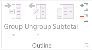
There are several potential reasons. Let’s get started
Solution 1: Only select one worksheet to group rows or columns
Have you selected several worksheets at the same time? In such case, you can’t add groupings. You can only do it sheet by sheet.
So, simply select one worksheet only. If that is not the reason, proceed with solution number 2 below.
Solution 2: You are editing a cell – just leave the cell to insert grouping
Are you inside an Excel cell, for example for typing a formula? If yes, you have to leave the cell first in order to add groupings. It’s also possible that you are editing a cell in a different Excel file (although in newer Excel versions that should not be a problem).
Do you want to boost your productivity in Excel?
Get the Professor Excel ribbon!

Add more than 120 great features to Excel!
Solution 3: Unprotect your worksheet or workbook to add grouping
The worksheet is protected? In that case you’d usually receive an error message. So, you have to unprotect a worksheet. In order to do that go to the Review ribbon and click on “Unprotect Sheet”.
Similar for downloaded Excel files: Excel opens these workbooks in the “Protected View” mode. You can see this with the yellow bar on top of your worksheet:
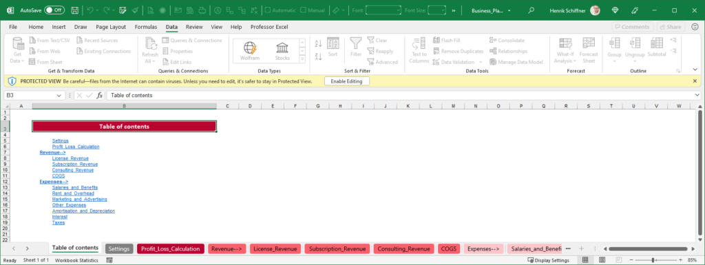
If you click on “Enable Editing”, you should be able to add a grouping.

Just a quick side note: Do you know that you can change the direction of groupings in Excel? Here is how to do that!
Solution 4: Show outline symbols within the Excel options
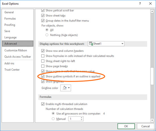
There also might be another reason. Within the Excel options, you can choose if you want to display groups. So maybe, the grouping works, but is just not shown?
- Click on “File” and the “Options”.
- Navigate to “Advanced” on the right-hand side and scroll down.
- Make sure the box “Show outline symbols if an outline is applied”.
- Confirm by clicking on “OK”.
Image by Michal Jarmoluk from Pixabay

Henrik Schiffner is a freelance business consultant and software developer. He lives and works in Hamburg, Germany. Besides being an Excel enthusiast he loves photography and sports.
Из этого руководства Вы узнаете и сможете научиться скрывать столбцы в Excel 2010-2013. Вы увидите, как работает стандартный функционал Excel для скрытия столбцов, а также научитесь группировать и разгруппировывать столбцы при помощи инструмента «Группировка».
Уметь скрывать столбцы в Excel очень полезно. Может быть множество причин не отображать на экране какую-то часть таблицы (листа):
- Необходимо сравнить два или более столбцов, но их разделяют несколько других столбцов. К примеру, Вы хотели бы сравнить столбцы A и Y, а для этого удобнее расположить их рядом. Кстати, в дополнение к этой теме, Вам может быть интересна статья Как закрепить области в Excel.
- Есть несколько вспомогательных столбцов с промежуточными расчётами или формулами, которые могут сбить с толку других пользователей.
- Вы хотели бы скрыть от посторонних глаз или защитить от редактирования некоторые важные формулы или информацию личного характера.
Читайте дальше, и вы узнаете, как Excel позволяет быстро и легко скрыть ненужные столбцы. Кроме того, из этой статьи Вы узнаете интересный способ скрыть столбцы с помощью инструмента «Группировка», который позволяет скрывать и отображать скрытые столбцы в одно действие.
- Скрываем выбранные столбцы в Excel
- Используем инструмент «Группировка», чтобы в один клик скрыть или отобразить столбцы
Скрываем выбранные столбцы в Excel
Вы хотите скрыть один или несколько столбцов в таблице? Есть простой способ сделать это:
- Откройте лист Excel и выделите столбцы, которые необходимо скрыть.
Подсказка: Чтобы выделить несмежные столбцы, отметьте их щелчком левой кнопки мыши при нажатой клавише Ctrl.
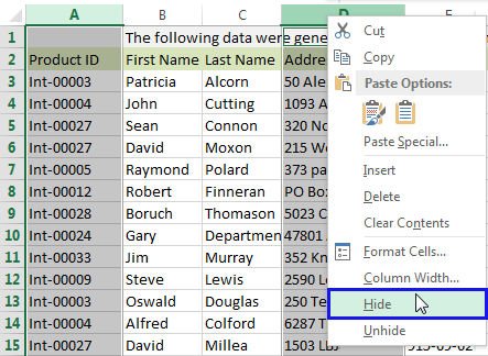
- Кликните правой кнопкой мыши на одном из выбранных столбцов, чтобы вызвать контекстное меню, и выберите Скрыть (Hide) из списка доступных действий.

Подсказка: Для тех, кто любит быстрые клавиши. Скрыть выделенные столбцы можно нажатием Ctrl+0.
Подсказка: Вы можете найти команду Скрыть (Hide) на Ленте меню Главная > Ячейки > Формат > Скрыть и отобразить (Home > Cells > Format > Hide & UnHide).
Вуаля! Теперь Вы с лёгкостью сможете оставить для просмотра только нужные данные, а не нужные скрыть, чтобы они не отвлекали от текущей задачи.
Используем инструмент «Группировка», чтобы в один клик скрыть или отобразить столбцы
Те, кто много работает с таблицами, часто используют возможность скрыть и отобразить столбцы. Существует ещё один инструмент, который отлично справляется с этой задачей, – Вы оцените его по достоинству! Этот инструмент – «Группировка». Бывает так, что на одном листе есть несколько несмежных групп столбцов, которые нужно иногда скрывать или отображать – и делать это снова и снова. В такой ситуации группировка значительно упрощает задачу.
Когда Вы группируете столбцы, сверху над ними появляется горизонтальная черта, показывающая, какие столбцы выбраны для группировки и могут быть скрыты. Рядом с чертой Вы увидите маленькие иконки, которые позволяют скрывать и отображать скрытые данные буквально в один клик. Увидев такие иконки на листе, Вы сразу поймёте, где находятся скрытые столбцы и какие столбцы могут быть скрыты. Как это делается:
- Откройте лист Excel.
- Выберите ячейки, которые надо скрыть.
- Нажмите Shift+Alt+Стрелка вправо.
- Появится диалоговое окно Группирование (Group). Выберите Колонны (Columns) и нажмите OK, чтобы подтвердить выбор.
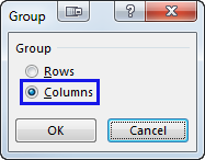
Подсказка: Еще один путь к этому же диалоговому окну: Данные > Группировать > Группировать (Data > Group > Group).

Подсказка: Чтобы отменить группировку выберите диапазон, содержащий сгруппированные столбцы, и нажмите Shift+Alt+Стрелка влево.
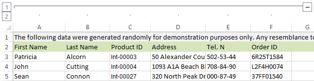
- Инструмент «Группировка» добавит специальные символы структуры на лист Excel, которые покажут какие именно столбцы входят в группу.
- Теперь по одному выделяйте столбцы, которые необходимо скрыть, и для каждого нажимайте Shift+Alt+Стрелка вправо.
Замечание: Объединить в группу можно только смежные столбцы. Если требуется скрыть несмежные столбцы, то придётся создавать отдельные группы.
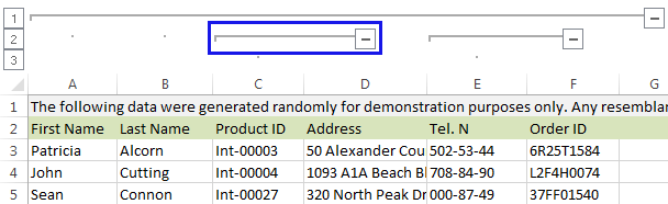
- Как только Вы нажмёте сочетание клавиш Shift+Alt+Стрелка вправо, скрытые столбцы будут показаны, а возле черты над сгруппированными столбцами появится специальная иконка со знаком «—» (минус).
- Нажатие на минус скроет столбцы, и «—» превратится в «+«. Нажатие на плюс моментально отобразит все скрытые в этой группе столбцы.
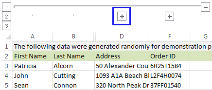
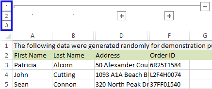
- После выполнении группировки в верхнем левом углу появляются маленькие цифры. Их можно использовать для того, чтобы скрывать и отображать одновременно все группы одинакового уровня. Например, в таблице, показанной ниже, нажатие на цифру 1 скроет все столбцы, которые видны на этом рисунке, а нажатие на цифру 2 скроет столбцы С и Е. Это очень удобно, когда Вы создаёте иерархию и несколько уровней группировки.
Вот и всё! Вы научились пользоваться инструментом для скрытия столбцов в Excel. Кроме того, Вы научились группировать и разгруппировывать столбцы. Надеемся, что знание этих хитростей поможет Вам сделать привычную работу в Excel гораздо проще.
Будьте успешны вместе с Excel!
Оцените качество статьи. Нам важно ваше мнение:
Most users are familiar with hiding rows or columns, but may not have ventured into grouping rows or columns.
What is the Group Function and How to Activate it?
The group function basically “ties a range (columns or rows, can’t be both) together, and allows you to collapse them (and expand them later), showing only the last row or column”. It is in the “Data” Ribbon, on the right in Excel 2007 and 2010.
After grouping the rows or columns, you can collaspe (basically, hide) them by pressing the “square minus” box on the left. To expand (basicaly, hide), press the “square plus”.
Shortcut:
Excel 2003: alt d g g
Excel 2007 or 2010: shift+alt+right (the Excel 2003 shortcut also works)

This is an example of a group of rows. The square buttons on the left and square brackets indicate which rows form the same group.
Uses and Advantages of Grouping Cells
The original purpose of grouping cells to group and hide details of various parts of big file with a data hierarchy, such as a budget. See below. The user can group and collapse (hide) all the details of each budget category all with a click of a button. This type of one click convenience is also why it is better than the normal hide function in many ways. (Hide needs 3 clicks for everything. On top of that, you have to make sure to highlight the correct rows or columns each time, where as grouping is just a click, and the same rows or columns are collapsed each time.) So the first advantage, and the biggest one, of using group is that it saves time and avoid errors.

Second advantage is that the group function can have multiple levels of hierarchies – something not possible with the normal hide or unhide function. Basically, the user can have nested groups, where they can hide and unhide the top group and not affect the subsequent bottom groups. See below for an example.

Third advantage is visibility. For fatigue users or when the user zoomed out on the spreadsheet, it is sometimes hard to see which row or columns are hidden. Group however, due to the expand “square plus” button, cues the user that there is more data underneath.
So, there it is. For those who hide / unhide cells for various purposes, such as formatting or just hiding tedious and unimportant details, I would definitely use group instead.
The One Drawback of Grouping Cells
One drawback is if you are dealing with multiple worksheets, and want to group the same rows / columns on multiple worksheets at the same time, it is basically not possible. In fact, the entire grouping / ungroup function does not work. Excel just won’t let you do it. You can, however, hide and unhide rows for multiple worksheets all at once. That is the one major I have encountered for grouping data instead of hiding it.
3 people found this article useful
3 people found this article useful
Get a handle on your data
Grouping rows and columns in Excel lets you collapse and expand sections of a worksheet. This can make large and complex datasets much easier to understand. Views become compact and organized. This article shows you step-by-step how to group and view your data.
Instructions in this article apply to Excel 2019, 2016, 2013, 2010, 2007; Excel for Microsoft 365, Excel Online and Excel for Mac.
Grouping in Excel
You can create groups by either manually selecting the rows and columns to include, or you can get Excel to automatically detect groups of data. Groups can also be nested inside other groups to create a multi-level hierarchy. Once your data is grouped, you can individually expand and collapse groups, or you can expand and collapse all groups at a given level in the hierarchy.
Groups provide a really useful way to navigate and view large and complex spreadsheets. They make it much easier to focus on the data that’s important. If you need to make sense of complex data you should definitely be using Groups and could also benefit from Power Pivot For Excel.
How to Use Excel to Group Rows Manually
To make Excel group rows, the simplest method is to first select the rows you want to include, then make them into a group.
-
For the group of rows you want to group, select the first row number and drag down to the last row number to select all the rows in the group.
-
Select the Data tab > Group > Group Rows, or simply select Group, depending on which version of Excel you’re using.
-
A thin line will appear to the left of the row numbers, indicating the extent of the grouped rows.
Select the minus (-) to collapse the group. Small boxes containing the numbers one and two also appear at the top of this region, indicating the worksheet now has two levels in its hierarchy: the groups and the individual rows within the groups.
-
The rows have been grouped and can now be collapsed and expanded as required. This makes it much easier to focus on just the relevant data.
How to Manually Group Columns in Excel
To make Excel group columns, the steps are almost the same as doing so for rows.
-
For the group of columns you want to group, select the first column letter and drag right to the last column letter, thereby selecting all the columns in the group.
-
Select the Data tab > Group > Group Columns, or select Group, depending on which version of Excel you’re using.
-
A thin line will appear above the column letters. This line indicates the extent of the grouped columns.
Select the minus (-) to collapse the group. Small boxes containing the numbers one and two also appear at the top of this region, indicating the worksheet now has two levels in its hierarchy for columns, as well as for rows.
-
The rows have been grouped and can now be collapsed and expanded as required.
How to Make Excel Group Columns and Rows Automatically
While you could repeat the above steps to create each group in your document, Excel can automatically detect groups of data and do it for you. Excel creates groups where formulas reference a continuous range of cells. If your worksheet doesn’t contain any formulas, Excel won’t be able to automatically create groups.
Select the Data tab > Group > Auto Outline and Excel will create the groups for you. In this example, Excel correctly identified each of the groups of rows. Because there’s no annual total for each spending category, it has not automatically grouped the columns.
This option isn’t available in Excel Online, if you’re using Excel Online, you’ll need to create groups manually.
How to Create a Multi-Level Group Hierarchy in Excel
In the previous example, categories of income and expense were grouped together. It would make sense to also group all of the data for each year. You can do this manually by applying the same steps as you used to create the first level of groups.
-
Select all of the rows to be included.
-
Select the Data tab > Group > Group Rows, or select Group, depending on which version of Excel you are using.
-
Another thin line will appear to the left of the lines representing the existing groups and indicating the extent of the new group of rows. The new group encompasses two of the existing groups and there are now three small numbered boxes at the top of this region, signifying the worksheet now has three levels in its hierarchy.
-
The spreadsheet now contains two levels of groups, with individual rows within the groups.
How to Automatically Create Multi-Level Hierarchy
Excel uses formulas to detect multi-level groups, just as it uses them to detect individual groups. If a formula references more than one of the other formulas which define groups, this indicates these groups are part of a parent group.
Keeping with the cash flow example, if we add a Gross Profit row to each year, which is simply the income minus the expenses, then this allows Excel to detect that each year is a group and the income and expenses are sub-groups within these. Select the Data tab > Group > Auto Outline to automatically create these multi-level groups.
How to Expand and Collapse Groups
The purpose of creating these groups of rows and/or columns is that it allows regions of the spreadsheet to be hidden, providing a clear overview of the entire spreadsheet.
-
To collapse all of the rows, select the number 1 box at the top of the region to the left of the row numbers.
-
Select the number two box to expand the first level of groups and make the second level of groups visible. The individual rows within the second level groups remain hidden.
-
Select the number three box to expand the second level of groups so the individual rows within these groups also become visible.
It’s also possible to expand and collapse individual groups. To do so, select the Plus (+) or Minus (-) that appears to mark a group that’s either collapsed or expanded. In this way, groups at different levels in the hierarchy can be viewed as required.
Thanks for letting us know!
Get the Latest Tech News Delivered Every Day
Subscribe