Excel not case sensitive

By definition, the VLOOKUP formula is not case-sensitive. Case-sensitive means, that it matters if you use capital letters or small letters. For instance, a VLOOKUP search for “AAA” will return the same value as for “aaa” or “Aaa”. But in some cases, you want to differentiate between capital and small letters. So how do you proceed? In this article, you learn how to make VLOOKUP, HLOOKUP, INDEX/MATCH and SUMIFS case-sensitive.

Example for all methods

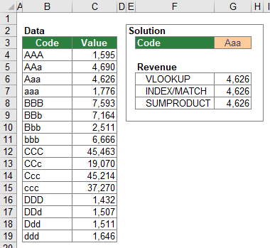
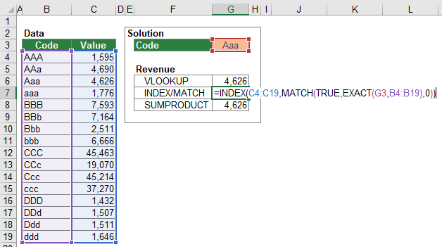
All following methods will be introduced with the example as shown in the image on the right-hand side. The cell range B4 to B19 contains codes (e.g. “AAA”, “AAa”, and so on) and the cell range C4 to C19 contains numeric values. In cell G3 you can insert a code (e.g. “Aaa”). The goal is to return the numeric value from the cells C4 to C19, depending on the code given in cell G3. For example if the code in G3 is “Aaa” you want to return the value from cell C6, which is 4,626.

Method 1a: Case-sensitive VLOOKUP

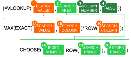
The first method is based on the VLOOKUP formula. Unfortunately, the approach is a little bit complex and only works through a workaround. The structure of the case-sensitive VLOOKUP is shown in the image on the right-hand side.

The underlying idea is not to conduct a VLOOKUP with the actual search value, but rather with the row number, in which the search value can be found.

1. SEARCH VALUE: This part of the formula identifies the row number. It comprises several formulas. The part EXACT()*ROW() returns an array of row numbers which match the search value. From this array, the embracing MAX formula just identifies the largest row number.
   1. SEARCH VALUE (within the EXACT formula): This is the actual value you look for.
   2. SEARCH COLUMN: The column you search in. It’s typically the leftmost column of your VLOOKUP formula.
   3. SEARCH COLUMN: Again, the same cell reference like the previous argument.
2. The SEARCH AREA creates an array (like a table with two columns) which contains the row numbers in the first column and the return values in the second column.
   1. INDEX NUMBER: In case of such lookup, the INDEX NUMBER is always {1,2}.
   2. SEARCH COLUMN: The range of cells in you search in as before in 1B and 1C.
   3. RETURN COLUMN: The column that contains the value you want to get returned.
3. The COLUMN NUMBER is in case of this exact VLOOKUP always 2. The reason is that from the virtual table created with the CHOOSE formula you need to return the value from the second column.
4. As usual, the last argument of the VLOOKUP formula is FALSE because you want search for the exact value.

Please note: As for all array formulas please press Ctrl + Shift + Enter on the keyboard after typing the formula.

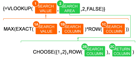
If you insert the fixed arguments into this formula, you get the simplified structure of the VLOOKUP formula in the image on the right-hand side.

For our example, the case-sensitive VLOOKUP has the following parameters:

• SEARCH VALUE: The search value is given in cell G3.
• SEARCH COLUMN: You search in the cell range B4 to B19.
• RETURN COLUMN: You want to get the value from cell range C4 to C19 returned.

Putting these parameters into the formula structure of Figure 93, you get the following formula.

{=VLOOKUP(MAX(EXACT(G3,B4:B19)*(ROW(B4:B19))),CHOOSE({1,2},ROW(B4:B19),C4:C19),2,0)}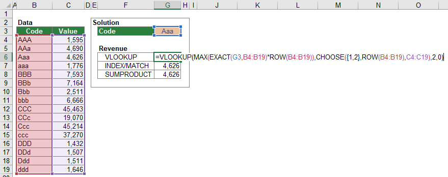

Method 1b: Case-sensitive HLOOKUP

A case-sensitive HLOOKUP works very similar to the VLOOKUP. The only difference is that you have to insert 3 TRANSPOSE formulas around and inside the CHOOSE formula. The reason is that CHOOSE can only handle vertical cell ranges in this case.

The structure of the case-sensitive HLOOKUP formula is shown in the image above. As you can see, the formula is getting quite long. This might be a good example for a possible solution in Excel, but not necessarily the best one. The following method number 2 is usually a better option for a case-sensitive, horizontal lookup.

The arguments of the HLOOKUP formula are pretty much the same as in method 1a, the VLOOKUP formula. Applying this to a very similar example leads to the following formula.

{=HLOOKUP(MAX(EXACT(D7,C3:R3)*COLUMN(C3:R3)),TRANSPOSE(CHOOSE({1,2},TRANSPOSE(COLUMN(C3:R3)),TRANSPOSE(C4:R4))),2,FALSE)}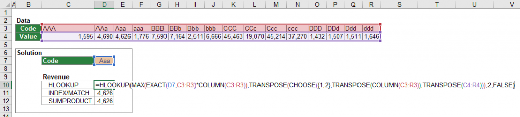

Method 2: Case-sensitive INDEX/MATCH

The case-sensitive INDEX/MATCH formula is compared to the case-sensitive VLOOKUP formula quite simple. The INDEX/MATCH formula is shorter and in many cases the better option.

The structure of the case-sensitive INDEX/MATCH formula combination is shown in the image on the right-hand side, the following number relate to the image.

1. RETURN RANGE: The range of cells containing the return value. This can be a vertical range (in case you use the INDEX/MATCH formula vertically) or a horizontal range of cells.
2. The LOOKUP VALUE is a little bit different than usual. Because the next argument (number 3) checks for each cell if it equals exactly (that means case-sensitive) the search value and returns an array of cells containing TRUE or FALSE for each cell, your LOOKUP VALUE is always TRUE for case-sensitive lookups.
3. The LOOKUP RANGE is usually the range of cells you search in for your lookup value. For a case-sensitive INDEX/MATCH formula combination, you create an array of cells (a virtual table) which contains only TRUE or FALSE. TRUE, if the SEARCH VALUE matches exactly the value of a cell in the SEARCH RANGE and FALSE, if not.
   1. The SEARCH VALUE is the value or cell reference you are looking for.
   2. The SEARCH RANGE contains the cells you are looking in.
4. Because you want to get an exact match, the last part of the MATCH formula is 0.

Please note (again): As for all array formulas please press Ctrl + Shift + Enter on the keyboard after typing the formula.

The structure shown in Figure 94 can be simplified. After inserting the fixed arguments, the INDEX/MATCH formula looks like in the image on the right-hand side.

Applying this structure on our example, you have the following parameters.

• RETURN RANGE: You want to return the value from the cell range C4 to C19.
• SEARCH VALUE: The search value is given in cell G3.
• SEARCH RANGE: You search in cell range B4 to B19.

If you now put these parameters into the structure, you get the following formula.

{=INDEX(C4:C11,MATCH(TRUE,EXACT(G3,B4:B11),0))}

Method 3: Case-sensitive SUMPRODUCT instead of SUMIFS

The SUMIFS formula doesn’t support an exact lookup. That’s why you could use an alternative formula instead: SUMPRODUCT. Although no “real” array formula (with curly brackets), the SUMPRODUCT formula works like an array formula because it deals with arrays.

The structure of the case-sensitive SUMPRODUCT formula is shown in the image above. The SUMPRODUCT formula multiplies all arguments with each other and sums up the results. If a criterion is not fulfilled, the argument is 0 so the result of the multiplication is 0.

• SEARCH VALUE: The value or cell reference you look for.
• SEARCH RANGE: The range of cells you look in.
• RETURN RANGE: The range of cells from which you want to get a value returned.

Because this formula is not an array formula, you don’t have to press Ctrl + Shift + Enter when finished typing.

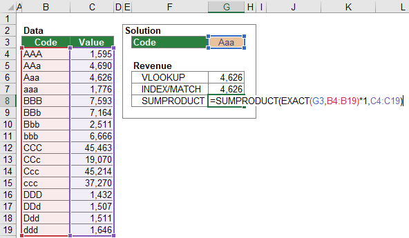
For the example of this chapter, you will get this SUMPRODUCT formula (also shown in the image on the right-hand side.

=SUMPRODUCT(EXACT(G3,B4:B19)*1,C4:C19)

Please note: The SUMPRODUCT approach only works with numeric return values (including dates). If your return value is a text or string, SUMPRODUCT doesn’t work.

Please feel free to download an Excel workbook with all the examples from this article. Just click on this link and the download starts immediately.

In this example, the goal is to perform a case-sensitive lookup on the name in column B, based on a lookup value entered in cell E5. By default, Excel is not case-sensitive. This means that standard lookup functions like VLOOKUP, XLOOKUP, and INDEX and MATCH are also not case-sensitive. These formulas will simply return the first match, ignoring upper and lower case. The classic way to work around this limitation is to build a lookup formula that incorporates the EXACT function, which performs a case-sensitive comparison. In a nutshell, we use the EXACT function to generate an array of TRUE and FALSE values, then alter the lookup formula to look for the first TRUE value. The article below explains how to use this approach with INDEX and MATCH, and XLOOKUP.

EXACT function

The EXACT function compares two text strings in a case-sensitive fashion. If the two strings are exactly the same, taking into account upper and lower case characters, EXACT returns TRUE. Otherwise, EXACT returns FALSE. For example:

=EXACT("apple","apple") // returns TRUE
=EXACT("Apple","apple") // returns FALSE

If we use the EXACT function on a range of values, we will get back multiple results. For example, if we use EXACT to compare the value in cell E5 with the range B5:B14:

EXACT(E5,B5:B14)

We get back an array that contains 10 TRUE and FALSE values like this:

{FALSE;FALSE;FALSE;FALSE;TRUE;FALSE;FALSE;FALSE;FALSE;FALSE}

This is because we are checking the name in E5 («JILL SMITH») against all 10 names in the range B5:B14. Notice the only TRUE value is in the 5th position. This corresponds to cell B9, which contains «JILL SMITH».

INDEX and MATCH solution

In the worksheet shown, the formula in cell F5 is:

=INDEX(C5:C14,MATCH(TRUE,EXACT(E5,B5:B14),0))

Working from the inside-out, EXACT is configured to compare the value in E5 against all names in the range B5:B14:

EXACT(E5,B5:B14) // returns 10 results

The EXACT function performs a case-sensitive comparison and returns TRUE or FALSE as a result. Because we are checking the name in E5 («JILL SMITH») against all 10 names in the range B5:B14, we get back an array of 10 TRUE and FALSE values like this:

{FALSE;FALSE;FALSE;FALSE;TRUE;FALSE;FALSE;FALSE;FALSE;FALSE}

This array is returned directly to the MATCH function as the lookup_array:

MATCH(TRUE,{FALSE;FALSE;FALSE;FALSE;TRUE;FALSE;FALSE;FALSE;FALSE;FALSE},0)

Notice the lookup_value given to MATCH is TRUE, and match_type is set to zero (0) to force an exact match. The lookup_array is created by the EXACT function. MATCH then returns 5, since the only TRUE in the array is at the fifth position. This result is returned directly to the INDEX function as the row number, so we can simplify the formula to:

=INDEX(C5:C14,5) // returns 39

With a row number of 5, INDEX returns the age in the fifth row (39) as a final result.

Note: this is an array formula and must be entered with Control + Shift + Enter in older versions of Excel.

XLOOKUP solution

The XLOOKUP function can be configured to perform a case-sensitive lookup using EXACT in the same way as INDEX and MATCH, but in a more compact formula:

=XLOOKUP(TRUE,EXACT(J5,B5:B14),C5:C14)

Notice the lookup_value and lookup_array are configured like the MATCH function above. After EXACT runs, we have the same array of 10 TRUE and FALSE values explained previously:

=XLOOKUP(TRUE,{FALSE;FALSE;FALSE;FALSE;TRUE;FALSE;FALSE;FALSE;FALSE;FALSE},C5:C14)

XLOOKUP returns the 5th item from the range C5:C14 (39) as a final result.

Note: For a more detailed example of a case-sensitive XLOOKUP formula, see this page.

Asked by: Darrell Koepp

Score: 4.9/5
(50 votes)

I guess every Excel user knows what function performs a vertical lookup in Excel. Right, it’s VLOOKUP. However, very few people are aware that Excel’s VLOOKUP is case-insensitive, meaning it treats lowercase and UPPERCASE letters as the same characters.

Is VLOOKUP format sensitive?

By default, the lookup value in the VLOOKUP function is not case sensitive. For example, if your lookup value is MATT, matt, or Matt, it’s all the same for the VLOOKUP function. It’ll return the first matching value irrespective of the case.

How do I ignore case sensitive in VLOOKUP?

Why you should never use VLOOKUP?

It can not lookup and return a value which is to the left of the lookup value. It works only with data which is arranged vertically. VLOOKUP would give a wrong result if you add/delete a new column in your data (as the column number value now refers to the wrong column).

Is Excel function case sensitive?

By default, Excel is not case-sensitive. For example, with «APPLE» in A1, and «apple» in A2, the following formula will return TRUE: =A1=A2 // returns TRUE To compare text strings in a case-sensitive way, you can… … Since MATCH alone isn’t case sensitive, we need a way to get Excel to compare case.

32 related questions found

VLOOKUP and INDEX-MATCH formulas are among the most powerful functions in Excel. Lookup formulas come in handy whenever you want to have Excel automatically return the price, product ID, address, or some other associated value from a table based on some lookup value. The VLOOKUP function can be used when the lookup value is in the left column of your table or when you want to return the last value in a column. The INDEX and MATCH functions can be used in combination to do the same thing, but provide greater flexibility without some of the limitations of VLOOKUP. I’ll also mention LOOKUP and CHOOSE and EXACT and ISBLANK and ISNUMBER and ISTEXT and … 🙂, but this article is mainly about VLOOKUP and INDEX-MATCH.

To see these examples in action, download the Excel file below.

Download the Example File (LookupFormulas.xlsx)

Do you have a VLOOKUP or INDEX-MATCH challenge you need to solve? If you can’t figure it out after reading this article, go ahead and ask your question by commenting below.

1) Simple VLOOKUP and INDEX-MATCH Examples

VLOOKUP Example

First, here is an example of the VLOOKUP function using a simple Price List Table. We’re looking for the text «a_003» within the Item ID column and wanting to return the corresponding value from the Price column.

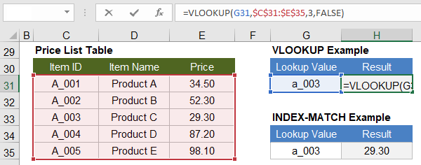
=VLOOKUP(lookup_value,table_array,col_index_num,FALSE)

How it works: The table_array argument is a range that must have the lookup column on the left. The price column is the 3rd column in the highlighted range, so that is why the col_index_num argument is 3 in our example. We use FALSE for the final argument because we want the VLOOKUP function to do an exact match.

INDEX-MATCH Example

Next, you’ll see that the INDEX-MATCH formula is just as simple:

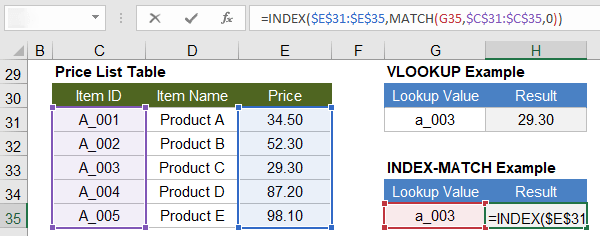
=INDEX(result_range,MATCH(lookup_value,lookup_range,0))

How it works: The MATCH function returns the position number 3 because «a_003» matches the 3rd row in the Item ID range. Next, INDEX(result_range,3) returns the 3rd value in the price list range.

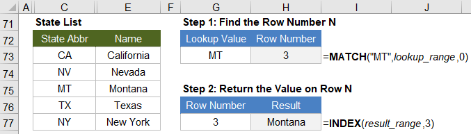
The INDEX-MATCH formula is an example of a simple nested function where we use the result from the MATCH function as one of the arguments for the INDEX function. The example below shows this being done in two separate steps.

Syntax and Notes for MATCH and INDEX

MATCH returns the position number of a matched value within the lookup range.

=MATCH(lookup_value,lookup_range,match_type)

INDEX returns a value from an array based on a row and column number.

=INDEX(array,row_number,[column_number],[area_number])

2) Use Wildcard Characters (?, *) for Partial Matches with VLOOKUP and INDEX-MATCH

Wildcard characters can be used within the lookup_value for both VLOOKUP and MATCH formulas when the lookup is text and you are doing an exact match.

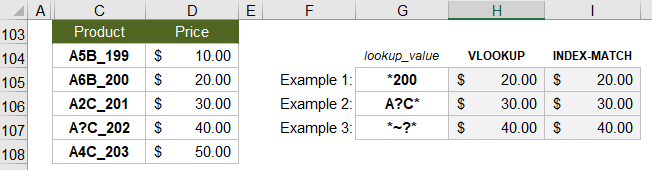
* (asterisk) matches any number of characters. For example, use «*200» to find the first value ending in 200.

? (question mark) matches any single character. For example, use «A?C*» to find the first value where «A» is the first character and «C» is the 3rd character. The second character can be anything, but only a single character.

~ (tilde) is used in front of a wildcard character to treat it as a literal character. In the 3rd example, we use «*~?*» to find the first occurrence of a product that contains an actual question mark.

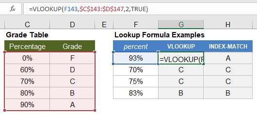
3) Return Approximate Matches Using VLOOKUP and INDEX-MATCH

The following examples show how to use VLOOKUP and INDEX-MATCH to return approximate matches with numerical lookup data. Important: When using an «Approximate Match» with VLOOKUP (where the 4th argument = TRUE) and a «Less than» match with MATCH (where the 3rd argument = 1), the lookup range needs to be sorted in ascending order.

These formulas look for the largest value that is less than or equal to the lookup value.

=VLOOKUP(lookup_value,table_array,col_index_num,TRUE)

=INDEX(result_range,MATCH(lookup_value,lookup_range,1))

Example 1: Return a Grade based on Percent

► See this in action: Download the Grade book Template

Example 2: Return a Discount Rate based on Quantity

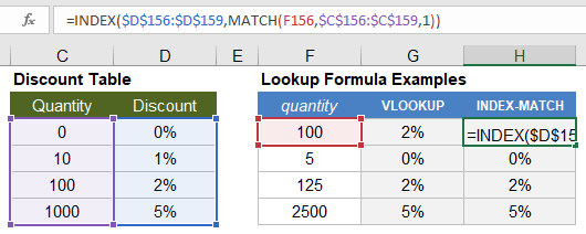
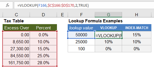
Example 3: Return a Tax Rate based on Income

► See this in action: Download the Paycheck Calculator

4) 2D Lookups Using VLOOKUP-MATCH and INDEX-MATCH-MATCH

In this example, we’ll do a mileage lookup between two cities. The formulas are basically the same as for a 1D lookup, except that we use a MATCH function to replace col_index_num in the VLOOKUP function and to replace column_number in the INDEX function.

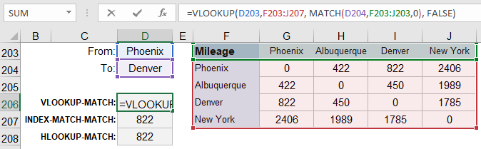
Using VLOOKUP

=VLOOKUP(row_lookup_value,table_array, MATCH(column_lookup_value,column_label_range,0), FALSE)

Using INDEX-MATCH-MATCH

=INDEX( result_array,
MATCH(row_lookup_value,row_label_range,0),
MATCH(column_lookup_value,column_label_range,0) )

Using HLOOKUP

=HLOOKUP(column_lookup_value,table_array, MATCH(row_lookup_value,row_label_range,0), FALSE)

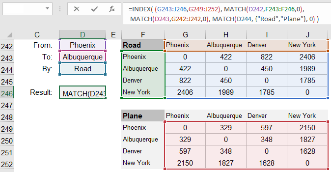
5) 3D Lookups Using INDEX-MATCH and VLOOKUP

To demonstrate a 3D lookup, we’ll use mileage tables again, but this time we have a separate table for Road and Plane. The INDEX function allows you to return a value from a 3D array. You can replace the row_number, column_number, and area_number with 3 MATCH functions.

NOTE The reference argument for the INDEX function should be multiple same-size ranges surrounded by parentheses like this: (A1:D10,E1:H10), or you can use a named range.

=INDEX( (array_range1,array_range2) ,
MATCH(row_lookup_value,row_label_range,0),
MATCH(column_lookup_value,column_label_range,0),
MATCH(table_lookup_value,{"Road","Plane"},0) )

3D Lookup Using VLOOKUP

It is possible to do a 3D lookup using VLOOKUP. Starting with the 2D lookup formula, in place of array_table, you can use CHOOSE(table_number,table_array_1,table_array_2). You can use MATCH to find the value for table_number as in the INDEX-MATCH example above. The resulting formula would look like this:

=VLOOKUP(row_lookup_value, CHOOSE( MATCH(table_name,{"Road","Plane"},0), road_table_array, plane_table_array), MATCH(column_lookup_value,column_label_range,0), FALSE)

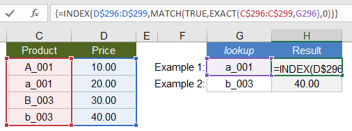
6) Case-Sensitive EXACT Lookup Using INDEX-MATCH

Most lookups and logical comparisons in Excel are NOT case-sensitive, meaning that both «A»=»a» and «A»=»A» would return TRUE.

The EXACT(value1,value2) function allows you to make a comparison between value1 and value2 that IS case sensitive, so EXACT(«A»,»a») returns FALSE and EXACT(«B»,»B») returns TRUE.

If you use EXACT to compare a value to a range like EXACT(«B»,A1:A20), the function returns an array of TRUE and FALSE values. You can then use a MATCH function to look for the value TRUE within the range returned by EXACT(lookup_value,lookup_range). The final lookup formula is an Excel Array Formula, so you need to press Ctrl+Shift+Enter after entering the formula.

{Ctrl+Shift+Enter} =INDEX(result_range, MATCH(TRUE,EXACT(lookup_value,lookup_range),0) )

See the references at the end of this article if you are curious about how a case-sensitive lookup can be done with VLOOKUP.

7) Multiple-Criteria Exact Lookups Using VLOOKUP and INDEX-MATCH

One way to do an exact-match using multiple criteria is to concatenate the lookup columns and do a lookup using the concatenated lookup values. VLOOKUP requires using a helper column containing the concatenated lookup columns. INDEX-MATCH does not need the helper column, but it becomes an array formula (Ctrl+Shift+Enter).

Multiple-criteria lookup using VLOOKUP and a helper column

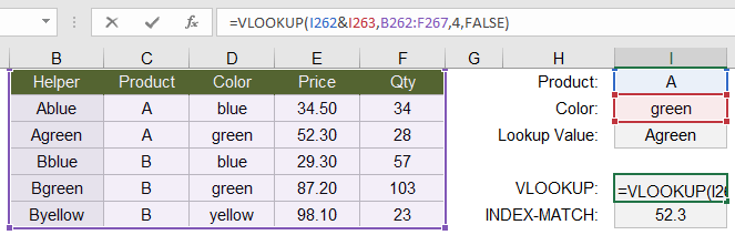
=VLOOKUP(value_1 & value_2,table_array,col_index_num,FALSE)

Multiple-criteria lookup using INDEX-MATCH as an array formula

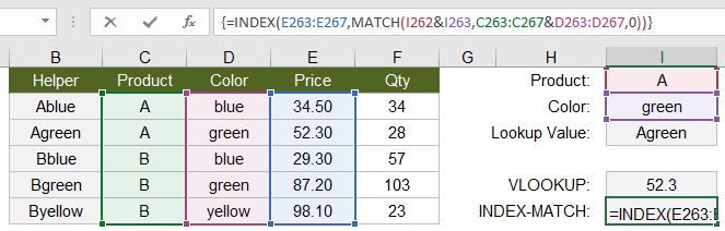
{Ctrl+Shift+Enter}  =INDEX(result_range,MATCH(value1 & value2, lookup_col1 & lookup_col2,0))

Lookups with Multiple Non-Exact Criteria Using INDEX-MATCH

When you want to use logical conditions such as A > B or A < B in your lookup, a method I like is to use INDEX-MATCH and convert the lookup_range to a TRUE or FALSE expression like lookup_range<lookup_value. Then search for the first occurrence of TRUE (using 1 as the first argument of the MATCH function). Using this method, you can have any number of conditions because multiplying true/false expressions together acts like the logical AND operator. The formula must be entered as an array formula (Ctrl+Shift+Enter), but that’s a small price to pay for relative simplicity.

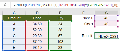
{Ctrl+Shift+Enter}  =INDEX(result_range,MATCH(1, (lookup_col1>lookup_value1) * (lookup_col2<lookup_value2) ,0) )

9) Return the Last Numeric Value in a Column

When using an approximate lookup for VLOOKUP and MATCH, you can return the last numeric value in a column if you use an extremely large number as the lookup value (to make sure it will be larger than any number in the lookup range). A common example would be to return the last value in a Balance column for a checkbook register as shown in the example below.

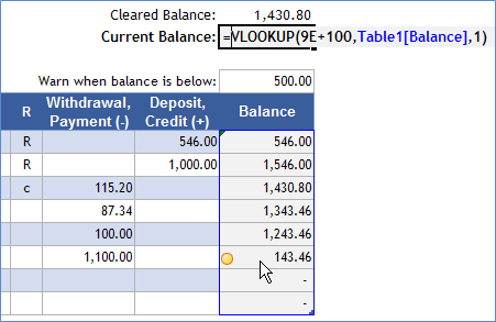
=VLOOKUP( 9E+100, lookup_column, 1, TRUE)

Recall that the TRUE option (for an approximate match) is the default for VLOOKUP, so that is why the formula in the checkbook example image only shows 3 arguments.

This can of course be done with INDEX-MATCH, but I prefer the VLOOKUP formula in this case because it requires only one reference to the lookup column.

=INDEX( lookup_column, MATCH( 9E+99, lookup_column, 1) )

NOTES The lookup_column can contain text values and even errors (like #N/A or #DIV/0), and those values will be ignored. The formula returns only the last numeric value.

10) Return the Last Text Value in a Column

When searching for the last text value, instead of a large numeric value for the lookup_value as in the previous example, use a «large» text value. By that, I mean a text value that would show up last if you sorted a column in alphabetical order. If you are using the English alphabet without special characters, that could be «zzzzzz.» If you are using Greek characters or symbols in your list, you could try a Unicode Character such as «🗿» as the lookup value.

=VLOOKUP( "zzzzzzz", lookup_column, 1, TRUE)

=INDEX( lookup_column, MATCH( "🗿", lookup_column, 1) )

Rather than returning the last text value, I often use just the MATCH part of this formula to return the row number of the last value. This allows you to make a dynamic named range that can be used as the source range for a drop-down list via data validation.

11) Return the Last Non-BLANK Value in a Column

If your column contains both text and numeric values, you may want a formula to return the last non-BLANK value. Using the INDEX-MATCH formula, we can search for the last numeric value and the last text value and return whichever comes last.

=INDEX( lookup_column, MAX( MATCH( "zzzzzz", lookup_column, 1), MATCH(9E+100, lookup_column,1) ) )

A more concise formula uses the LOOKUP function. The LOOKUP function allows the lookup_range to be an expression rather than a direct reference (and it can be a row or column). We can use a logical comparison and search for the last TRUE value like this:

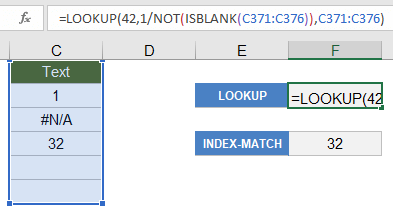
=LOOKUP(42, 1/NOT(ISBLANK(lookup_range)), lookup_range)

The trick here is that the expression 1/NOT(ISBLANK(lookup_range)) returns an array of 1s for TRUE and #DIV/0 errors for FALSE. LOOKUP ignores the error values so it will return the last value in lookup_range that is not blank. The number 42 is arbitrary — it just needs to be larger than 1 to return the last value.

Using very similar formulas, you can use LOOKUP to return just the last numeric value or text value like this:

=LOOKUP( 42, 1/ISNUMBER(lookup_range), result_range)

=LOOKUP( 42, 1/ISTEXT(lookup_range), result_range)

12) Return the Last Non-Empty Value Using LOOKUP

If you are using a formula to return an empty value «» and you want to ignore those cells when searching for the last value in the range, you can use the LOOKUP formula mentioned in the last example with the expression 1/(lookup_range<>»»).

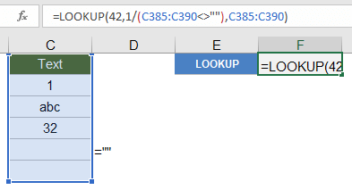
=LOOKUP(42, 1/(lookup_range<>""), lookup_range)

If you want to return the relative row number instead of the actual value, you can use the following formula:

=LOOKUP(42, 1/(lookup_range<>""), ROW(lookup_range)-ROW(first_cell_in_lookup_range)+1 )

13) Lookup based on the Nth Match

You can use the SMALL function to return the Nth smallest value from an array, and we can use that along with an array formula and the INDEX function to do a lookup based on the Nth match. See my Array Formula Examples article to learn more about Array Formulas and specifically the SMALL-IF formula.

In this example, we want to return the 2nd Event that matches the date 3/7/2018. Note: The curly { } brackets in the formula below are a reminder to press Ctrl+Shift+Enter to enter the formula as an Array Formula. You don’t actually type the brackets into the formula.

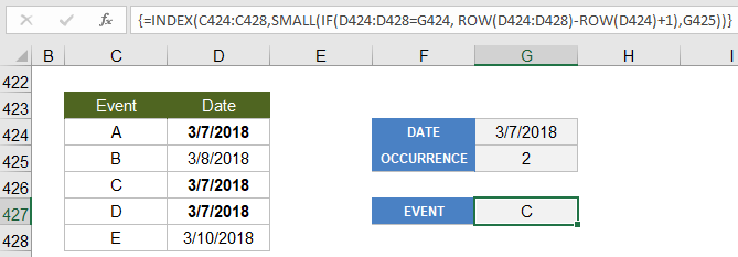
{  =INDEX(result_range,SMALL( IF(lookup_range=lookup_value, ROW(lookup_range)-ROW(first_cell_in_lookup_range)+1),occurrence))  }

How does this work? The SMALL-IF part of the formula is acting kind of like the MATCH function except that it is returning the index number for the 2nd occurrence of the match. We can use SMALL in this example because Excel stores dates as numbers.

This formula is used within the Daily Planner Template to list events and holidays occurring on a particular date.

14) VLOOKUP vs. INDEX-MATCH

Excel people like to debate about whether VLOOKUP is better than INDEX-MATCH for lookup formulas. The most common argument is that VLOOKUP is simpler and INDEX-MATCH is more powerful. Even though I usually prefer INDEX-MATCH, I think both formulas are pretty simple, and one isn’t necessarily always more powerful than the other.

If you want to do more advanced lookups with VLOOKUP, then you’ll probably need to learn how to use MATCH and CHOOSE. If you want to become a power Excel user, then you’ll also want to learn the INDEX function. So, my opinion on the VLOOKUP vs. INDEX-MATCH debate is to learn how to use them all.

In conclusion, here are some reminders applicable to both VLOOKUP and INDEX-MATCH:

• Don’t forget the FALSE or 0 option if you are wanting an exact match, because the default parameter is to use an approximate match.
• As a general rule, use absolute ($A$1) cell references to refer to the lookup ranges and table arrays because when you copy the lookup formula you will usually want those ranges to remain the same.
• Check for extra blank spaces if you think a lookup formula should be finding a match, but it is not.
• Use IFERROR to handle the error returned when an exact match is not found.

References