
Every once in a while, you might find Excel behaving in a bizarre or unexpected way. One example is when you accidentally trigger the scroll lock feature. Another example is when one or more formulas suddenly stops working. Instead of a result, you see only a formula, as in the screen below:

The VLOOKUP formula is correct, why no result?
This can be very confusing, and you might think you’ve somehow broken your spreadsheet. However, it’s likely a simple problem. With a little troubleshooting, you can get things working again. There are two main reasons you might see a formula instead of a result:
- You accidentally enabled Show Formulas
- Excel thinks your formula is text
I’ll walk through each case with some examples.
Show Formulas is enabled
Excel has a feature called Show Formulas that toggles the display of formula results and actual formulas. Show Formulas is meant to give you a quick way to see all formulas in a worksheet. However, if you accidentally trigger this mode, it can be quite disorienting. With Show Formulas enabled, columns are expanded, and every formula in a worksheet is displayed with no results anywhere in sight, as shown below.

Show Formulas disabled (normal mode)

Show Formulas enabled
To check if Show Formulas is turned on, visit the Formula tab in the ribbon and check the Show Formulas button:

Show Formulas enabled — just click to disable
The reason Show Formulas can be accidentally enabled is because it has a keyboard shortcut (Control +`) that a user might accidentally type. Try typing Control + ` in a worksheet to see how it works. You should see formulas toggled on and off each time you use the shortcut.
Show Formulas toggles the display of every formula in a worksheet. If you are having trouble with a single formula, the problem isn’t Show Formulas. Instead, Excel probably thinks the formula is text. Read on for more information.
Excel thinks your formula is text
If Excel thinks a formula is just text, and not an actual formula, it will simply display the text without trying to evaluate it as a formula. There are several situations that might cause this behavior.
No equal sign
First, you may have forgotten the equal sign. All formulas in Excel must begin with an equal sign (=). If you leave this out, Excel will simply treat the formula as text:

Broken formula example — no equal sign (=)
Space before equal sign
A subtle variation of this problem can occur if there is one or more spaces before the equal sign. A single space can be hard to spot, but it breaks the rule that all formulas must start with an equal sign, so it will break the formula as shown below:

Formula wrapped in quotes
Finally, make sure the formula is not wrapped in quotes. Sometimes, when people mention a formula online, they will use quotes, like this:
"=A1"
In Excel, quotes are used to signify text, so the formula will not be evaluated, as seen below:

Note: you are free to use quotes inside formulas. In this case, the formula above requires quotes around criteria.
In all of the examples above, just edit the formula so it begins with an equal sign and all should be well:

For reference, here is the working formula:
=SUMIFS(D5:D9,E5:E9,">30")
Cell format set to Text
Finally, every once in a while, you might see a formula that is well-formed in every way, but somehow does not display a result. If you run into a formula like this, check to see if the cell format is set to Text.

If so, set the format to General, or another suitable number format. You may need to enter cell edit mode (click into the formula bar, or use F2, then enter) to get Excel to recognize the format change. Excel should then evaluate as a formula.
Tip — Save formula in progress as text
Although a broken formula is never fun, you can sometimes use the «formula as text problem» to your advantage, as a way to save work in progress on a tricky formula. Normally, if you try to enter a formula in an unfinished state, Excel will throw an error, stopping you from entering the formula. However, if you add a single apostrophe before the equal sign Excel will treat the formula as text and let you enter without complaint. The single quote reminds you that the formula has been intentionally converted to text:

Later, you can then come back later to work on the formula again, starting where you left off. See #17 in this list for more info.
Summary: Is your Excel spreadsheet showing text of a formula you’ve entered and not its result? This blog explains the possible reasons behind such an issue. Also, it describes solutions to fix the ‘Excel formula not showing result’ error. You can try Stellar Repair for Excel software to recover engineering and shared formulas.

Contents
- Why Does Excel Show or Display the Formula Not the Result?
- How to Fix ‘Excel Showing Formula Not Result’ Issue?
- What to Do If the Manual Solutions Don’t Work?
- Conclusion
Sometimes, when you type a formula in a cell of worksheet and press Enter, instead of showing the calculated result, it returns the formula as text. For instance, Excel cell shows:

But you should get the result as:

Why Does Excel Show or Display the Formula Not the Result?
Following are the possible reasons that may lead to the ‘Excel showing formula not result’ issue:
- You accidentally enabled “Show Formulas” in Excel.
- The cell format in a spreadsheet is set to text.
- ‘Automatic calculation’ feature in Excel is set to manual.
- Excel thinks your formula is text (Syntax are not followed).
- You type numbers in a cell with unnecessary formatting.
How to Fix ‘Excel Showing Formula Not Result’ Issue?
Here are some solutions to fix the issue:
Solution 1 – Disable Show Formulas
If only formula shows in Excel not result, check if you have accidentally or intentionally enabled ‘show formula’ feature of Excel. Instead of applying calculations and then showing results, this feature displays the actual text written by you.
You can use the ‘Show Formulas’ feature to quickly view all formulas, but if you are not aware of this feature, and enabled it accidentally, it can be a headache. To disable this mode, go to ‘Formulas’ and click on ‘Show formula enabled.’ If it’s previously enabled, it will be disabled by just clicking on it.

Solution 2 – Cell Format Set to Text
Another possible reason that only formula shows in Excel not result could be that the cell format is set to text. This means that anything written in any format in that cell will be treated as regular text. If so, change the format to General or any other. To get Excel to recognize the change in the format, you may need to enter cell edit mode by clicking into the formula bar or just press F2.

Solution 3 – Change Calculation Options from ‘Manual’ to ‘Automatic’
There is an “automatic calculation” feature in Excel, which tells Excel to do calculations automatically or manually. If ‘Excel formula is not showing results’, it may be because the automatic calculations feature is set to manual. This issue is not easily detected because it results in calculating formula in one cell but if you copy it to some other cell, it will retain the first calculation and will not recalculate on the base of the new location. To fix this, follow these steps:
- In Excel, click on the ‘File’ tab on the top left corner of the screen.
- In the window that opens, click on ‘Options’ from the left menu bar.
- From ‘Excel Options’ dialog box, select ‘Formulas’ from the left side menu and then change the ‘Calculation options’ to ‘Automatic’ if it’s currently set as ‘Manual’.

- Click on ‘OK’. This will redirect you to your sheet.
Solution 4 – Type Formula in the Right Format
There is a proper way to tell Excel that your text is a formula. If you don’t write the formula in a particular format, Excel considers it as simple text and hence no calculations are performed according to it. For this reason, keep the following in mind when typing a formula:
- Equal sign: Every formula in Excel should start with an equal sign (=). If you miss it, Excel will mistake your formula as regular text.
- Space before equal sign: You are not supposed to enter any space before equal sign. Maybe a single space will be hard for us to detect, but it breaks the rule of writing formulas for Excel.
- Formula wrapped in quotes: You need to make sure that your formula is not wrapped in quotes. People usually make this mistake of writing a formula in quotes, but in Excel, quotes are used to signify text. So your formula won’t be evaluated. But you can add quotes inside formula if required, for example: =SUMIFS(F5:F9,G5:G9,”>30″).
- Match all parentheses in a formula: Arguments of Excel functions are entered in parenthesis. In complex cases, you may need to enter more sets of parenthesis. If those parentheses are not paired/closed properly, Excel may not be able to evaluate the entered formula.
- Nesting limit: If you are nesting two or more Excel functions into each other, for example using nested IF loop, remember the following rules:
- Excel 2019, 2016, 2013, 2010, and 2007 versions only allow to use up to 64 nested functions.
- Excel 2003 and lower versions only allow up to 7 nested functions.
Solution 5 – Enter Numbers without any Formatting
When you use a number in the formula, make sure you don’t enter any decimal separator or currency sign, e.g. $, etc. In an Excel formula, a comma is used to separate arguments of a function and a dollar sign makes an absolute cell reference. Most of these special characters have built-in functions so avoid using them unnecessarily.
What to Do If the Manual Solutions Don’t Work?
If you’ve tried out the manual solutions mentioned above but still unable to resolve the ‘Excel formula not showing result’ issue, you can try repairing your Excel file with the help of an automated Excel repair software, such as Stellar Repair for Excel.
This reliable and competent software scans and repairs Excel files (.XLSX and .XLS). It also helps recover all the file components, like formulas, cell formatting, etc. Armed with an interactive GUI, this software is extremely easy to work with, and its advanced algorithms allow it to fend off Excel errors with ease.
Conclusion
This blog outlined the possible reasons that may cause ‘Excel not showing formula results’ issue. Check out these reasons and implement the manual fixes, depending on what resulted in the problem in the first place. If none of these fixes help resolve the issue, corruption in the Excel file might be preventing the formulas from showing the actual results. In that case, using Stellar Excel Repair tool might help.
About The Author
Priyanka
Priyanka is a technology expert working for key technology domains that revolve around Data Recovery and related software’s. She got expertise on related subjects like SQL Database, Access Database, QuickBooks, and Microsoft Excel. Loves to write on different technology and data recovery subjects on regular basis. Technology freak who always found exploring neo-tech subjects, when not writing, research is something that keeps her going in life.
Best Selling Products

Stellar Repair for Excel
Stellar Repair for Excel software provid
Read More

Stellar Toolkit for File Repair
Microsoft office file repair toolkit to
Read More

Stellar Repair for QuickBooks ® Software
The most advanced tool to repair severel
Read More

Stellar Repair for Access
Powerful tool, widely trusted by users &
Read More
I’m working on an excel sheet and I’ve encountered an issue I’ve never come across before. I’m trying to sum the results of an array function, but I’m not getting any results from the sum on the sheet — just blank cells. The weird part is when I press F9 in the formula bar it shows the correct summed value that should show in the cells on the sheet. I just don’t get why the value would appear in the formula bar, but not in the cells on the sheet. Other forums mentioned changing the calculation option (on automatic of course) or to ‘show zeros’, which just changed the cells to zero instead of blank. F9 still shows the correct value. Here’s the formula:
{=SUM(OFFSET(INDIRECT("Sheet1!E"&IF(ISERROR(MATCH($A$2:$A$15&$C$1,Sheet1!$C$2:$C$51,0)),
1000,MATCH($A$2:$A$15&$C$1,Sheet1!$C$2:$C$51,0))),0,ROW(1:1)))}
The match gets me the row index for the numbers I need to sum. (E1000 is just a default for when there isn’t a match and references a cell with 0 in it). If I remove the sum from the function and use F9 I can see the actual array with the numbers to be summed. This is what is so confusing to me. Everything seems to evaluate correctly, it just doesn’t show on the sheet. Thanks for the help!
![]()
Xavier Guihot
52.1k21 gold badges284 silver badges183 bronze badges
asked Apr 28, 2016 at 7:29
![]()
6
I know this thread is a couple months old, but for anyone having this issue, try checking for Circular References. It is likely that your formula has at least one.
To check: click the Formulas tab, click the arrow next to Error Checking, point to Circular References, and then click the first cell listed in the submenu.
Reasoning: When using the Evaluate Formula function (F9), it only does a one time calculation and is able to give a complete result. However, if a circular reference is present, the formula in the sheet itself will continuously recalculate so may never have a definitive result.
answered Dec 11, 2016 at 19:33
![]()
3
I came here because I had the same issue, and the above did not initially work for me.
I found that to execute the array function you must highlight the entire formula and then (for Mac) press Control+Shift+Enter.
Once I did this it worked like a charm!!
![]()
Xavier Guihot
52.1k21 gold badges284 silver badges183 bronze badges
answered Mar 15, 2018 at 3:31
![]()
Joann Joann
111 bronze badge
1
Try «Recalculate All» on the formulas tab.
This solved a similar issue for me with an AVERAGEIF function, whose value would show up correctly in the formula viewer, but not in the sheet. Forcing the sheet to recalculate everything fixed the problem in my case.
The problem seems to occur when defining a cell that is based on another cell, that is based on other cells, that are based on other cells, that are based on other cells…at some point Excel seems to give up and assume that there’s a circular reference somewhere, even though there isn’t in my case.
When Excel calculates all sheets, it re-uses results, and ignores cells until their precedents are known, rather than working backward from a particular cell, so it doesn’t freak out if a cell relies on too many preceding cells.
answered Sep 7, 2018 at 3:59
![]()
Theodore MurdockTheodore Murdock
1,5181 gold badge13 silver badges27 bronze badges
Having the same problem, very frustrating. I have found an insane solution. I don’t know why it works but it does… I thought that I would try the formula in another cell. So I copied and pasted the cell in another cell… And the formula in the original cell worked and the correct value appeared.
![]()
answered Jul 5, 2016 at 0:28
![]()
1
I came across this problem when using SUMIFS with three queries on an array. I found the solution was to encapsulate the whole function in brackets. I think the problem must arise from the order in which excel evaluates the constituents of the formula when it derives its answer.
So for example I had to add the following brackets [highlighted in bold] =
SUMIFS( [00_COMBINED_NO_DUPLICATES.xlsx]COMBINED!$CK$2:$CK$60067,
        [00_COMBINED_NO_DUPLICATES.xlsx]COMBINED!$F$2:$F$60067,
        [@RR1],
        [00_COMBINED_NO_DUPLICATES.xlsx]COMBINED!$S$2:$S$60067,
        ">="&[@[Quarter_Starting]],
        [00_COMBINED_NO_DUPLICATES.xlsx]COMBINED!$S$2:$S$60067,
        "<"&EOMONTH([@[Quarter_Starting]],
        2
      )+1)
![]()
ρяσѕρєя K
132k52 gold badges197 silver badges213 bronze badges
answered Feb 1, 2017 at 0:20
![]()
AkanniAkanni
9249 silver badges10 bronze badges
This was happening to me. I solved it by pressing Ctrl and ‘
OR you can go to View, and unselect Show formulas.
In ‘normal’ Excel Ctrl+’ would insert the data from the cell above.
Hope this helps someone.
answered May 8, 2017 at 13:21
![]()
Make Calculate option as automatic. It should solve the probelem
See the screen shot
answered Jun 13, 2017 at 9:29
![]()
Sorry to reopen this but here is a new solution.
I do have circular references, deliberately, so I set Excel to allow them to evaluate only once. Default is OFF — do not evaluate, hence why your formulae returned false / 0 every time even if they appeared true.
To switch on Iterative calculations (i.e. do something with circular references instead of nothing): File -> Options -> Formulas -> Enable Iterative Calculations -> Change from 100 (a little excessive except in special applications) to 1.
Link (scroll down to the bit about iterative calculations): https://support.office.com/en-ie/article/remove-or-allow-a-circular-reference-8540bd0f-6e97-4483-bcf7-1b49cd50d123
Hope this helps some more folks!
answered Mar 27, 2019 at 12:34
![]()
jfgoodhew1jfgoodhew1
952 silver badges11 bronze badges
Sometimes it is a problem if you are using arrays with OFFSET or INDIRECT.
You can solve it using =N(INDIRECT(… or =N(OFFSET(
You can find the explanation below
Array Formula Confusion
answered Jun 22, 2020 at 18:56
![]()
Many of us have old ways to correct the formula, but let me tell you something: The iterative formula which shows correct results using «F9» means that you do not have to check the formula again and again.
You also do not have to check except the type=»general» — that’s it.
Now please please, please allow FILE>OPTIONS>FORMULAS>ENABLE ITERATIVE CALCULATION, maximum iteration = 300 (assuming you have 300 cells for iteration), maximum change = 0.001.
This is because we have to check whether the iteration is allowed or not. Hope your problem gets solved.
![]()
ouflak
2,44810 gold badges44 silver badges49 bronze badges
answered Oct 30, 2021 at 17:47
![]()
This problem also occurred when using an excel table reference. Converting the table to normal cells fixed it. Alternatively, changing the references from table to normal references fixed it too.
This part of a formula caused a #value / #wert error
VERGLEICH(LF5;DATWERT('Inzidenz RKI_20211129.xlsx'!Table6[[#Kopfzeilen];[27.09.2021]:[26.11.2021]]);0)
This did not:
VERGLEICH(LF5;DATWERT('[Inzidenz RKI_20211129.xlsx]LK_7-Tage-Fallzahl-aktualisiert'!$C$3:$C$173);0)
(vergleich is match, and datwert is datevalue in german excel, and it uses ; instead of commas)
answered Nov 29, 2021 at 7:08
![]()
DrWhatDrWhat
2,3305 gold badges19 silver badges31 bronze badges
Возможности Excel позволяют выполнять расчеты любой сложности благодаря формулам и функциям. Однако иногда пользователи могут обнаружить, что формула не работает или выдает ошибку вместо желаемого результата. В этой статье мы рассмотрим, почему это происходит, и какие действия нужно предпринять для устранения проблемы.
Решение 1: меняем формат ячеек
Очень часто Excel отказывается выполнять вычисления из-за неправильного формата ячеек.
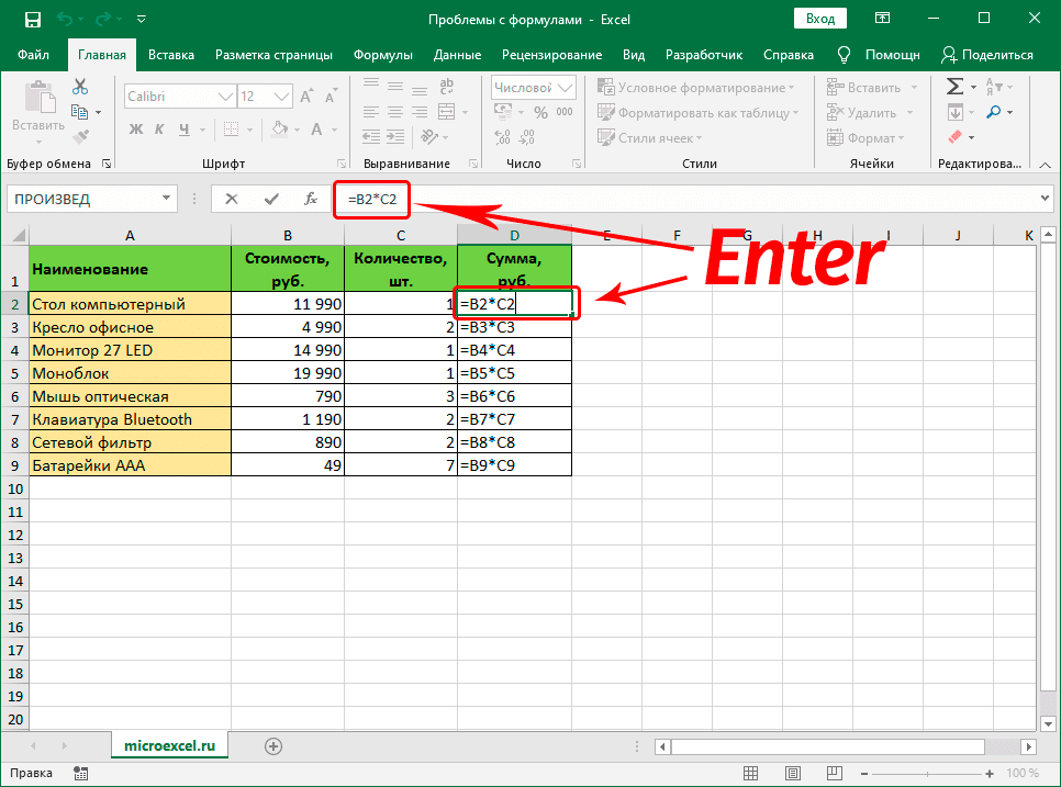
Например, если задан текстовый формат, то вместо результата мы увидим только саму формулу в виде простого текста.
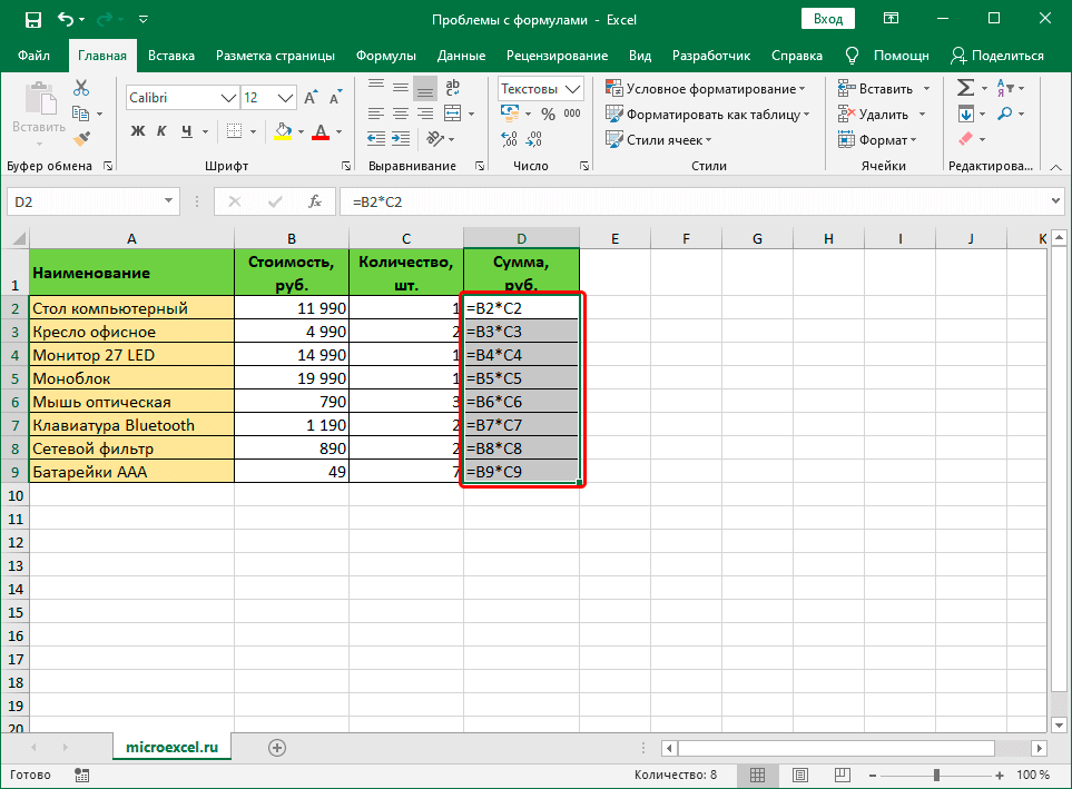
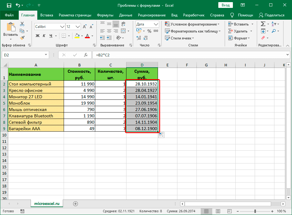
В некоторых ситуациях при выборе неправильного формата результат можно рассчитать, но он будет отображаться совершенно иначе, чем хотелось бы.
Очевидно, что формат ячейки нужно изменить, и это делается следующим образом:
- Чтобы определить текущий формат ячейки (диапазон ячеек), выделите его и, находясь на вкладке «Главная», обратите внимание на группу инструментов «Число». Здесь есть специальное поле, которое показывает используемый сейчас формат.

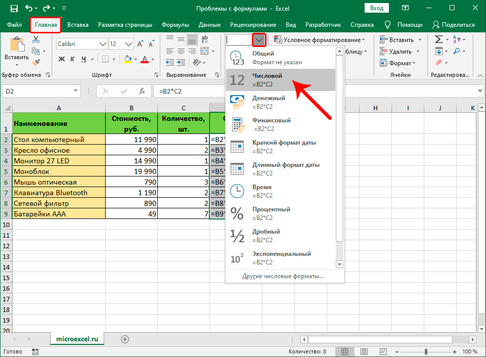
- Вы можете выбрать другой формат из списка, который откроется после нажатия стрелки вниз рядом с текущим значением.

Формат ячейки можно изменить с помощью другого инструмента, который позволяет выполнять более сложные настройки.
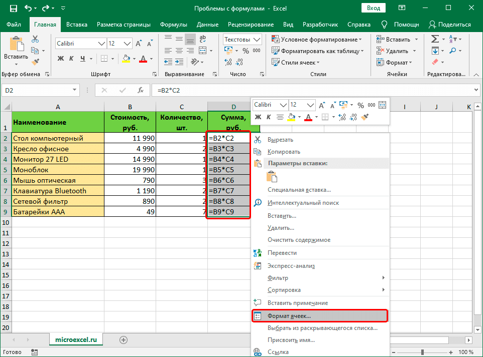
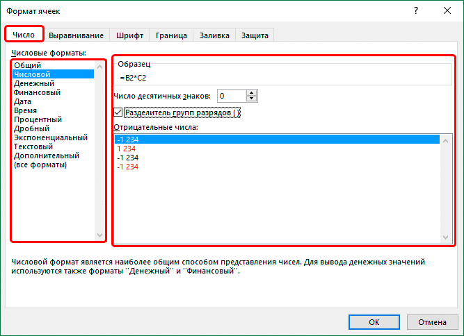
- После выбора ячейки (или выбора диапазона ячеек) щелкните ее правой кнопкой мыши и в открывшемся списке выберите команду «Форматировать ячейки». Или вместо этого после выделения нажмите Ctrl + 1.
- В открывшемся окне мы окажемся во вкладке «Номер». Здесь, в списке слева, находятся все доступные форматы, из которых мы можем выбирать. Слева отображаются настройки выбранной опции, которые мы можем изменить по своему усмотрению. Когда все будет готово, нажмите ОК.
- Чтобы изменения отразились в таблице, по очереди включите режим редактирования для всех ячеек, в которых формула не сработала. После выбора желаемого элемента вы можете продолжить изменение, нажав клавишу F2, дважды щелкнув по нему или щелкнув внутри строки формул. Затем, ничего не меняя, нажмите Enter.
Примечание. Если данных слишком много, на выполнение последнего шага вручную потребуется много времени. В этом случае можно поступить иначе — использовать маркер заливки. Но это работает только тогда, когда одна и та же формула используется во всех ячейках.
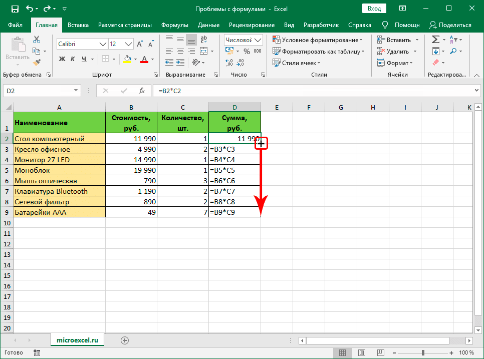
- Последний шаг выполняем только для верхней ячейки. Затем перемещаем указатель мыши в ее нижний правый угол, как только появится черный знак плюса, удерживая левую кнопку мыши и перетаскивая ее в конец таблицы.
- Получаем столбец с результатами, рассчитанными по формулам.

Решение 2: отключаем режим “Показать формулы”
Когда мы видим сами формулы вместо результатов, это может быть связано с тем, что режим отображения формул включен и его нужно выключить.
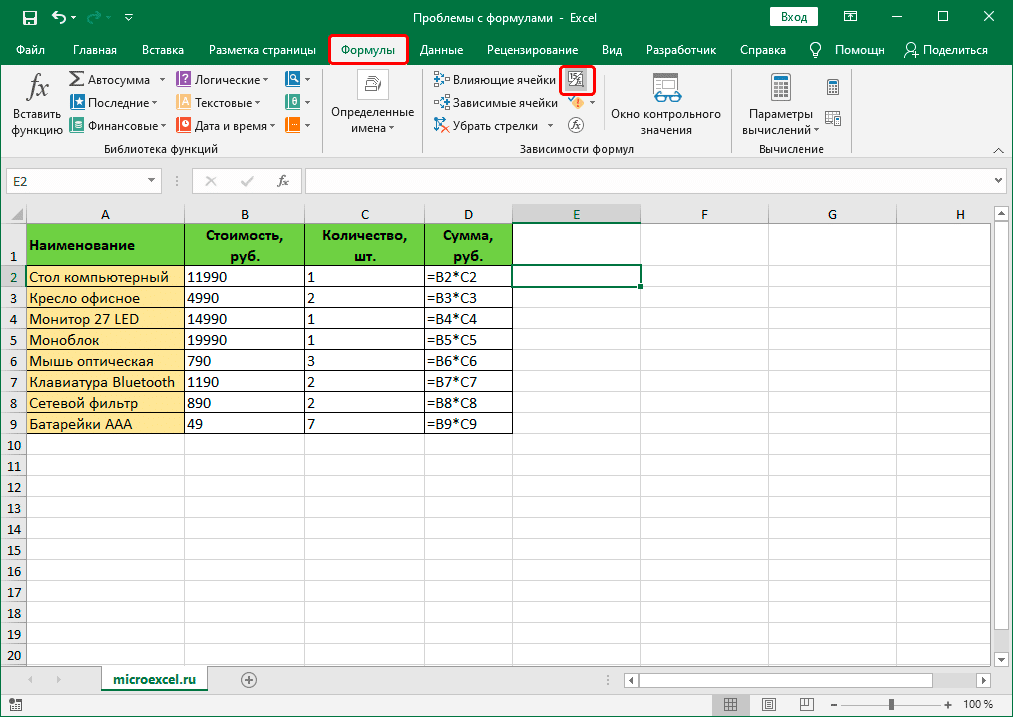
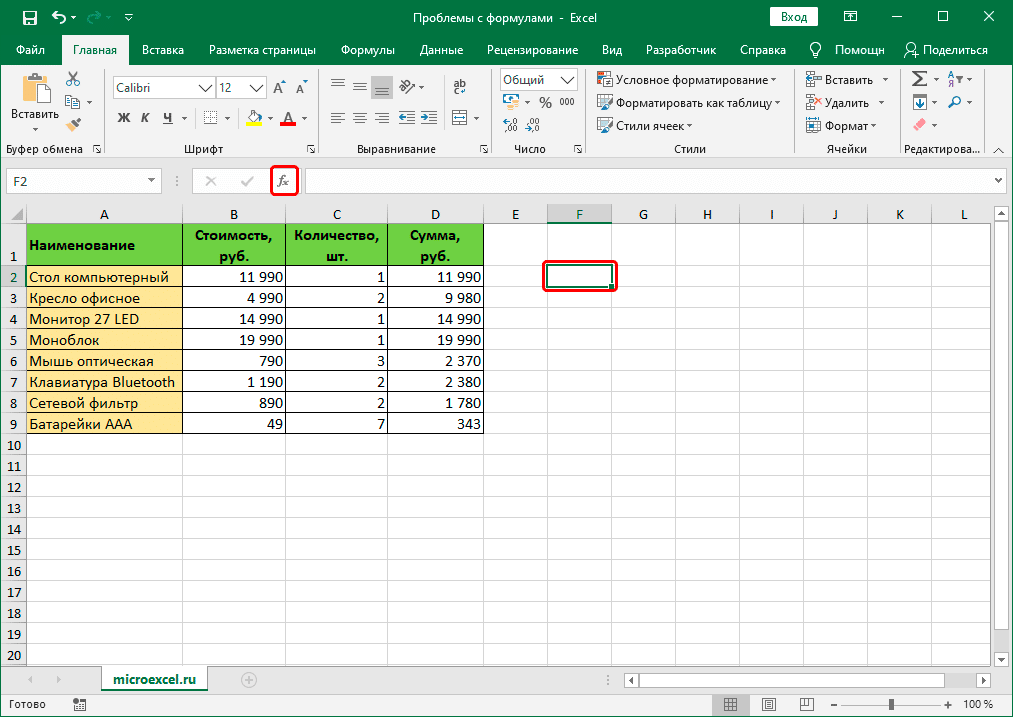
- Перейдите на вкладку «Формулы». На панели инструментов «Зависимость формул» нажмите кнопку «Показать формулы», если она активна.
- В результате результаты расчета теперь будут отображаться в ячейках с формулами. Правда, из-за этого могут меняться границы столбцов, но это решаемо.
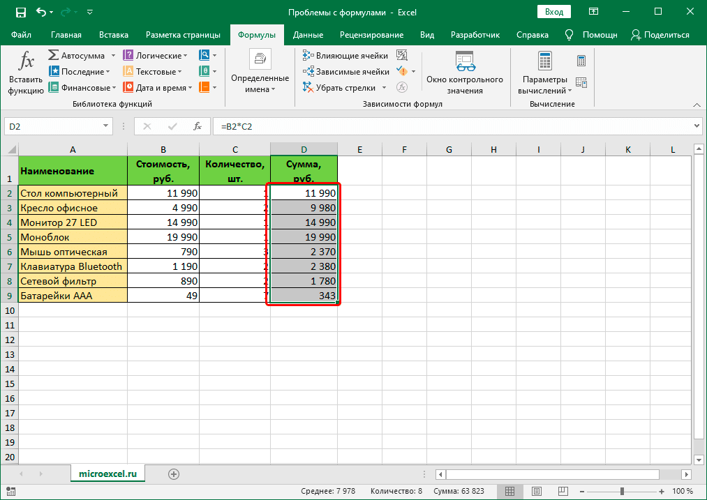
Решение 3: активируем автоматический пересчет формул
Иногда может возникнуть ситуация, когда формула вычислила какой-то результат, однако, если мы решим изменить значение в одной из ячеек, на которые ссылается формула, пересчет не будет выполнен. Это решается в параметрах программы.
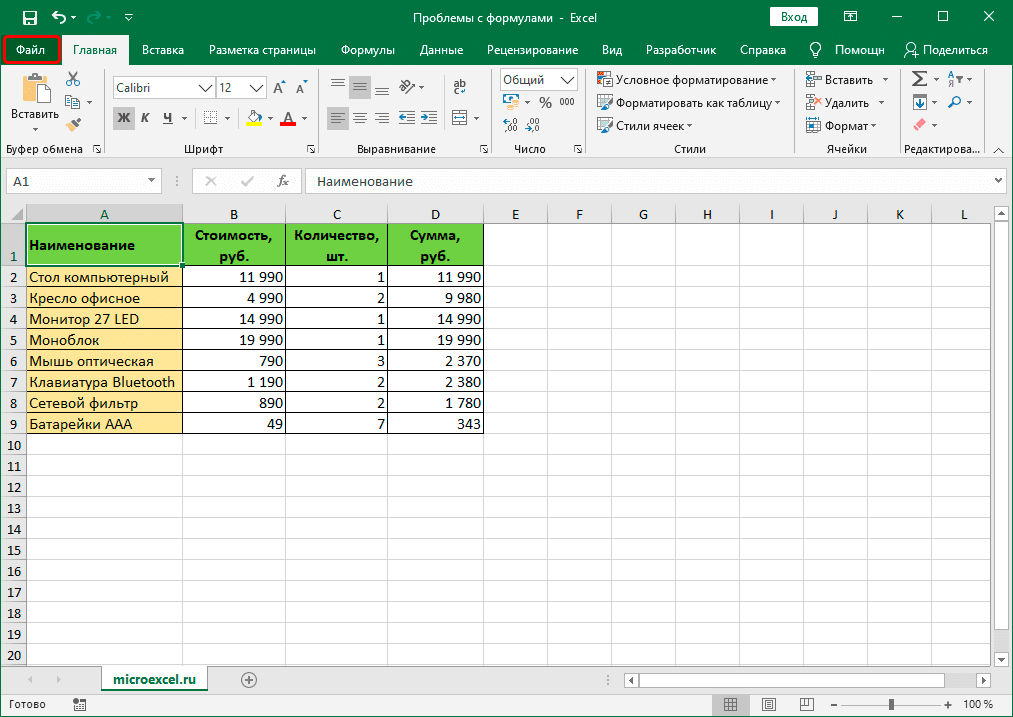
- Зайдите в меню «Файл”.
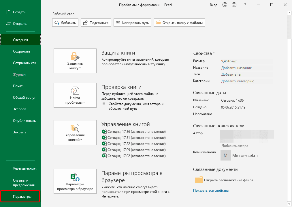
- В списке слева выберите раздел «Параметры”.
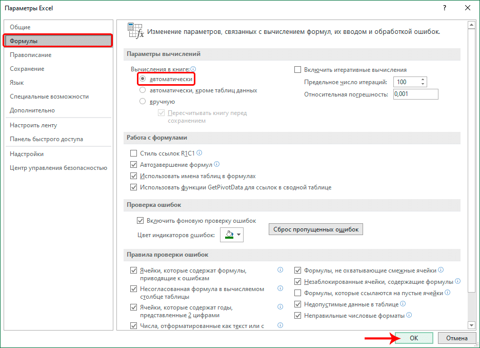
- В появившемся окне перейдите в подраздел «Формулы». В правой части окна в группе «Параметры расчета» поставьте галочку напротив опции «автоматический», если выбран другой вариант. Когда все будет готово, нажмите ОК.
- Все готово, с этого момента все результаты по формулам будут автоматически пересчитаны.
Решение 4: исправляем ошибки в формуле
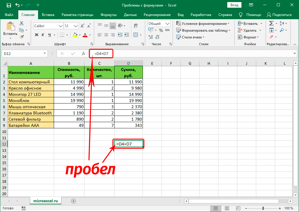
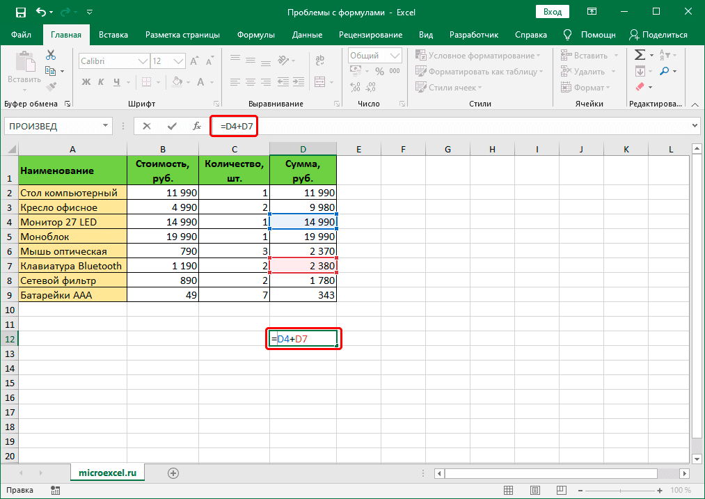
Если вы ошиблись в формуле, программа может воспринять ее как простое текстовое значение, поэтому вычисления по ней производиться не будут. Например, одна из самых распространенных ошибок — это пробел перед знаком равенства. При этом помните, что знак «=» обязательно должен предшествовать любой формуле.
Также очень часто допускаются ошибки в синтаксисе функций, поскольку их не всегда легко ввести, особенно когда используется несколько аргументов. Поэтому рекомендуется использовать мастер функций для вставки функции в ячейку.
Чтобы формула работала, просто внимательно проверьте ее и исправьте обнаруженные ошибки. В нашем случае вам просто нужно удалить пробел в начале, что не обязательно.
Иногда проще стереть формулу и переписать ее, чем пытаться найти ошибку в уже написанной. То же самое верно для функций и их аргументов.
Распространенные ошибки
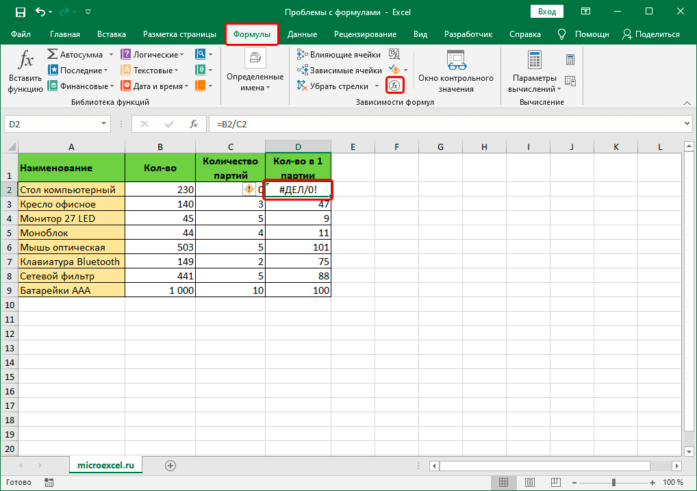
В некоторых случаях, когда пользователь допустил ошибку при вводе формулы, в ячейке могут отображаться следующие значения:
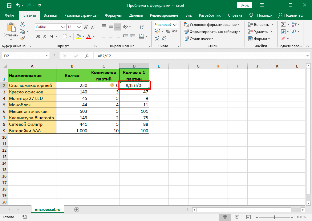
- # DIV / 0! — результат деления на ноль;
- # N / A — введите недопустимые значения;
- #КОЛИЧЕСТВО! — неверное числовое значение;
- #ЦЕНИТЬ! — в функции использован неверный тип аргумента;
- # ПУСТОЙ! — неверный адрес диапазона;
- #СВЯЗЬ! — ячейка, к которой относится формула, удалена;
- #ИМЯ? — Имя недопустимо в формуле.
Если мы видим любую из вышеперечисленных ошибок, в первую очередь проверяем, правильно ли заполнены все данные в ячейках, участвующих в формуле. Затем проверяем саму формулу и наличие в ней ошибок, в том числе противоречащих законам математики. Например, деление на ноль недопустимо (ошибка # DIV / 0!).
В случаях, когда вам нужно иметь сложные функции, которые ссылаются на множество ячеек, вы можете использовать инструменты проверки.
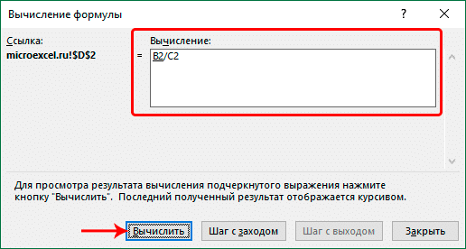
- Мы отмечаем ячейку, содержащую ошибку. На вкладке «Формулы» в группе инструментов «Зависимости формул» нажмите кнопку «Вычислить формулу”.
- В открывшемся окне отобразится подробная информация о расчете. Для этого нажмите кнопку «Рассчитать» (каждое нажатие переходит к следующему шагу).
- Таким образом, вы можете отслеживать каждый шаг, находить ошибку и исправлять ее.
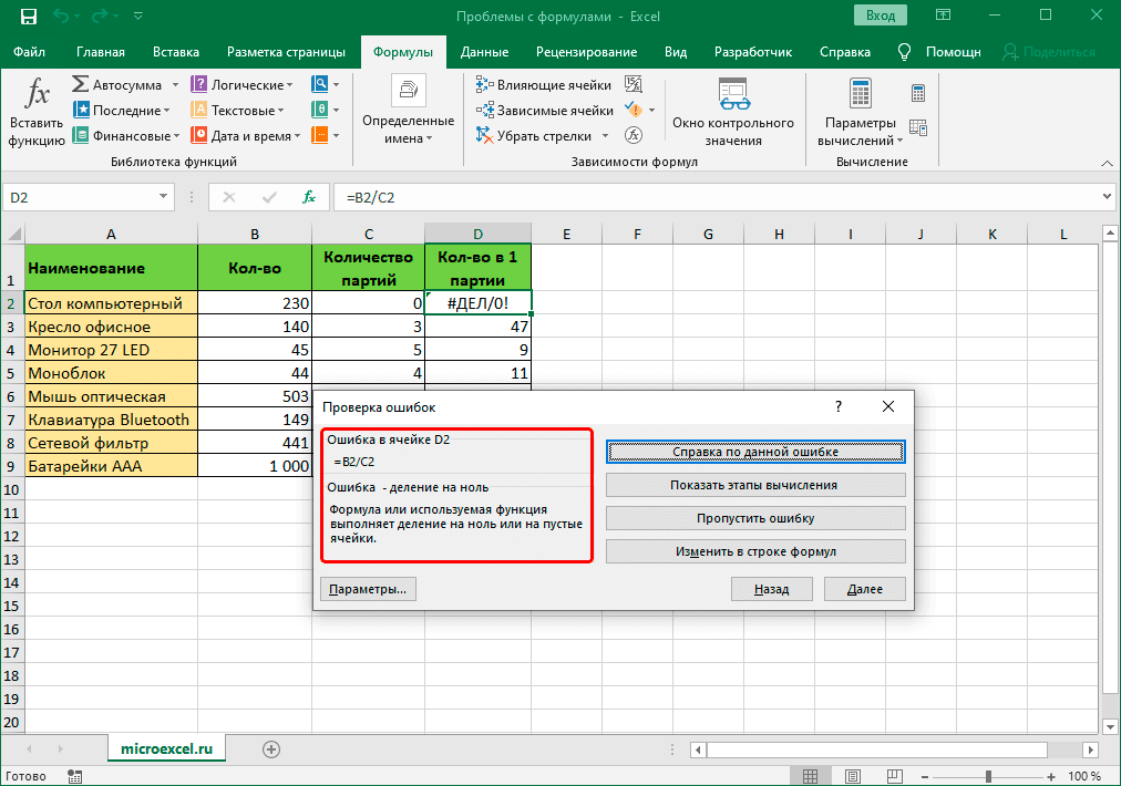
Вы также можете использовать полезный инструмент проверки ошибок, расположенный в том же блоке.
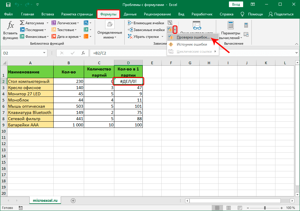
Откроется окно, в котором будет описана причина ошибки и предложен ряд действий в этом отношении, включая исправление в строке формул.
Заключение
Работа с формулами и функциями — одна из основных возможностей Excel и, несомненно, одно из основных направлений использования программы. Поэтому очень важно знать, какие проблемы могут возникнуть при работе с формулами и как их решать.