
Name a cell
-
Select a cell.
-
In the Name Box, type a name.

-
Press Enter.
To reference this value in another table, type th equal sign (=) and the Name, then select Enter.
Define names from a selected range
-
Select the range you want to name, including the row or column labels.
-
Select Formulas > Create from Selection.
-
In the Create Names from Selection dialog box, designate the location that contains the labels by selecting the Top row, Left column, Bottom row, or Right column check box.
-
Select OK.
Excel names the cells based on the labels in the range you designated.
Use names in formulas
-
Select a cell and enter a formula.
-
Place the cursor where you want to use the name in that formula.
-
Type the first letter of the name, and select the name from the list that appears.
Or, select Formulas > Use in Formula and select the name you want to use.
-
Press Enter.
Manage names in your workbook with Name Manager
-
On the ribbon, go to Formulas > Name Manager. You can then create, edit, delete, and find all the names used in the workbook.
Name a cell
-
Select a cell.
-
In the Name Box, type a name.
-
Press Enter.
Define names from a selected range
-
Select the range you want to name, including the row or column labels.
-
Select Formulas > Create from Selection.
-
In the Create Names from Selection dialog box, designate the location that contains the labels by selecting the Top row,Left column, Bottom row, or Right column check box.
-
Select OK.
Excel names the cells based on the labels in the range you designated.
Use names in formulas
-
Select a cell and enter a formula.
-
Place the cursor where you want to use the name in that formula.
-
Type the first letter of the name, and select the name from the list that appears.
Or, select Formulas > Use in Formula and select the name you want to use.
-
Press Enter.
Manage names in your workbook with Name Manager
-
On the Ribbon, go to Formulas > Defined Names > Name Manager. You can then create, edit, delete, and find all the names used in the workbook.
In Excel for the web, you can use the named ranges you’ve defined in Excel for Windows or Mac. Select a name from the Name Box to go to the range’s location, or use the Named Range in a formula.
For now, creating a new Named Range in Excel for the web is not available.
What’s in the name?
If you are working with Excel spreadsheets, it could mean a lot of time saving and efficiency.
In this tutorial, you’ll learn how to create Named Ranges in Excel and how to use it to save time.
Named Ranges in Excel – An Introduction
If someone has to call me or refer to me, they will use my name (instead of saying a male is staying in so and so place with so and so height and weight).
Right?
Similarly, in Excel, you can give a name to a cell or a range of cells.
Now, instead of using the cell reference (such as A1 or A1:A10), you can simply use the name that you assigned to it.
For example, suppose you have a data set as shown below:
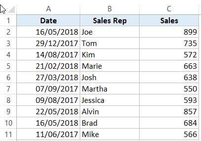
In this data set, if you have to refer to the range that has the Date, you will have to use A2:A11 in formulas. Similarly, for Sales Rep and Sales, you will have to use B2:B11 and C2:C11.
While it’s alright when you only have a couple of data points, but in case you huge complex data sets, using cell references to refer to data could be time-consuming.
Excel Named Ranges makes it easy to refer to data sets in Excel.
You can create a named range in Excel for each data category, and then use that name instead of the cell references. For example, dates can be named ‘Date’, Sales Rep data can be named ‘SalesRep’ and sales data can be named ‘Sales’.

You can also create a name for a single cell. For example, if you have the sales commission percentage in a cell, you can name that cell as ‘Commission’.
Benefits of Creating Named Ranges in Excel
Here are the benefits of using named ranges in Excel.
Use Names instead of Cell References
When you create Named Ranges in Excel, you can use these names instead of the cell references.
For example, you can use =SUM(SALES) instead of =SUM(C2:C11) for the above data set.
Have a look at ṭhe formulas listed below. Instead of using cell references, I have used the Named Ranges.
- Number of sales with value more than 500: =COUNTIF(Sales,”>500″)
- Sum of all the sales done by Tom: =SUMIF(SalesRep,”Tom”,Sales)
- Commission earned by Joe (sales by Joe multiplied by commission percentage):
=SUMIF(SalesRep,”Joe”,Sales)*Commission
You would agree that these formulas are easy to create and easy to understand (especially when you share it with someone else or revisit it yourself.
No Need to Go Back to the Dataset to Select Cells
Another significant benefit of using Named Ranges in Excel is that you don’t need to go back and select the cell ranges.
You can just type a couple of alphabets of that named range and Excel will show the matching named ranges (as shown below):

Named Ranges Make Formulas Dynamic
By using Named Ranges in Excel, you can make Excel formulas dynamic.
For example, in the case of sales commission, instead of using the value 2.5%, you can use the Named Range.
Now, if your company later decides to increase the commission to 3%, you can simply update the Named Range, and all the calculation would automatically update to reflect the new commission.
How to Create Named Ranges in Excel
Here are three ways to create Named Ranges in Excel:
Method #1 – Using Define Name
Here are the steps to create Named Ranges in Excel using Define Name:
This will create a Named Range SALESREP.
Method #2: Using the Name Box
- Select the range for which you want to create a name (do not select headers).
- Go to the Name Box on the left of Formula bar and Type the name of the with which you want to create the Named Range.

- Note that the Name created here will be available for the entire Workbook. If you wish to restrict it to a worksheet, use Method 1.
Method #3: Using Create From Selection Option
This is the recommended way when you have data in tabular form, and you want to create named range for each column/row.
For example, in the dataset below, if you want to quickly create three named ranges (Date, Sales_Rep, and Sales), then you can use the method shown below.
Here are the steps to quickly create named ranges from a dataset:
This will create three Named Ranges – Date, Sales_Rep, and Sales.
Note that it automatically picks up names from the headers. If there are any space between words, it inserts an underscore (as you can’t have spaces in named ranges).
Naming Convention for Named Ranges in Excel
There are certain naming rules you need to know while creating Named Ranges in Excel:
- The first character of a Named Range should be a letter and underscore character(_), or a backslash(). If it’s anything else, it will show an error. The remaining characters can be letters, numbers, special characters, period, or underscore.
- You can not use names that also represent cell references in Excel. For example, you can’t use AB1 as it is also a cell reference.
- You can’t use spaces while creating named ranges. For example, you can’t have Sales Rep as a named range. If you want to combine two words and create a Named Range, use an underscore, period or uppercase characters to create it. For example, you can have Sales_Rep, SalesRep, or SalesRep.
- While creating named ranges, Excel treats uppercase and lowercase the same way. For example, if you create a named range SALES, then you will not be able to create another named range such as ‘sales’ or ‘Sales’.
- A Named Range can be up to 255 characters long.
Too Many Named Ranges in Excel? Don’t Worry
Sometimes in large data sets and complex models, you may end up creating a lot of Named Ranges in Excel.
What if you don’t remember the name of the Named Range you created?
Don’t worry – here are some useful tips.
Getting the Names of All the Named Ranges
Here are the steps to get a list of all the named ranges you created:
This will give you a list of all the Named Ranges in that workbook. To use a named range (in formulas or a cell), double click on it.

Displaying the Matching Named Ranges
- If you have some idea about the Name, type a few initial characters, and Excel will show a drop down of the matching names.


How to Edit Named Ranges in Excel
If you have already created a Named Range, you can edit it using the following steps:
Useful Named Range Shortcuts (the Power of F3)
Here are some useful keyboard shortcuts that will come handy when you are working with Named Ranges in Excel:
- To get a list of all the Named Ranges and pasting it in Formula: F3
- To create new name using Name Manager Dialogue Box: Control + F3
- To create Named Ranges from Selection: Control + Shift + F3
Creating Dynamic Named Ranges in Excel
So far in this tutorial, we have created static Named Ranges.
This means that these Named Ranges would always refer to the same dataset.
For example, if A1:A10 has been named as ‘Sales’, it would always refer to A1:A10.
If you add more sales data, then you would have to manually go and update the reference in the named range.
In the world of ever-expanding data sets, this may end up taking up a lot of your time. Every time you get new data, you may have to update the Named Ranges in Excel.
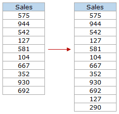
To tackle this issue, we can create Dynamic Named Ranges in Excel that would automatically account for additional data and include it in the existing Named Range.
For example, For example, if I add two additional sales data points, a dynamic named range would automatically refer to A1:A12.
This kind of Dynamic Named Range can be created by using Excel INDEX function. Instead of specifying the cell references while creating the Named Range, we specify the formula. The formula automatically updated when the data is added or deleted.
Let’s see how to create Dynamic Named Ranges in Excel.
Suppose we have the sales data in cell A2:A11.

Here are the steps to create Dynamic Named Ranges in Excel:
-
- Go to the Formula tab and click on Define Name.

- In the New Name dialogue box type the following:
- Name: Sales
- Scope: Workbook
- Refers to: =$A$2:INDEX($A$2:$A$100,COUNTIF($A$2:$A$100,”<>”&””))

- Click OK.
- Go to the Formula tab and click on Define Name.


Done!
You now have a dynamic named range with the name ‘Sales’. This would automatically update whenever you add data to it or remove data from it.
How does Dynamic Named Ranges Work?
To explain how this work, you need to know a bit more about Excel INDEX function.
Most people use INDEX to return a value from a list based on the row and column number.
But the INDEX function also has another side to it.
It can be used to return a cell reference when it is used as a part of a cell reference.
For example, here is the formula that we have used to create a dynamic named range:
=$A$2:INDEX($A$2:$A$100,COUNTIF($A$2:$A$100,"<>"&""))
INDEX($A$2:$A$100,COUNTIF($A$2:$A$100,”<>”&””) –> This part of the formula is expected to return a value (which would be the 10th value from the list, considering there are ten items).
However, when used in front of a reference (=$A$2:INDEX($A$2:$A$100,COUNTIF($A$2:$A$100,”<>”&””))) it returns the reference to the cell instead of the value.
Hence, here it returns =$A$2:$A$11
If we add two additional values to the sales column, it would then return =$A$2:$A$13
When you add new data to the list, Excel COUNTIF function returns the number of non-blank cells in the data. This number is used by the INDEX function to fetch the cell reference of the last item in the list.
Note:
- This would only work if there are no blank cells in the data.
- In the example taken above, I have assigned a large number of cells (A2:A100) for the Named Range formula. You can adjust this based on your data set.
You can also use OFFSET function to create a Dynamic Named Ranges in Excel, however, since OFFSET function is volatile, it may lead a slow Excel workbook. INDEX, on the other hand, is semi-volatile, which makes it a better choice to create Dynamic Named Ranges in Excel.
You may also like the following Excel resources:
- Free Excel Templates.
- Free Online Excel Training (7-Part Online Video Course).
- Useful Excel Macro Code Examples.
- 10 Advanced Excel VLOOKUP Examples.
- Creating a Drop Down List in Excel.
- Creating a Named Range in Google Sheets.
- How to Reference Another Sheet or Workbook in Excel
- How to Delete Named Range in Excel?
Named ranges are one of these crusty old features in Excel that few users understand. New users may find them weird and scary, and even old hands may avoid them because they seem pointless and complex.
But named ranges are actually a pretty cool feature. They can make formulas *a lot* easier to create, read, and maintain. And as a bonus, they make formulas easier to reuse (more portable).
In fact, I use named ranges all the time when testing and prototyping formulas. They help me get formulas working faster. I also use named ranges because I’m lazy, and don’t like typing in complex references 
The basics of named ranges in Excel
What is a named range?
A named range is just a human-readable name for a range of cells in Excel. For example, if I name the range A1:A100 «data», I can use MAX to get the maximum value with a simple formula:
=MAX(data) // max value

The beauty of named ranges is that you can use meaningful names in your formulas without thinking about cell references. Once you have a named range, just use it just like a cell reference. All of these formulas are valid with the named range «data»:
=MAX(data) // max value
=MIN(data) // min value
=COUNT(data) // total values
=AVERAGE(data) // min value
Video: How to create a named range
Creating a named range is easy
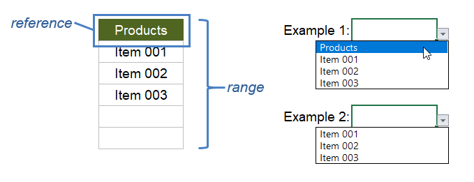
Creating a named range is fast and easy. Just select a range of cells, and type a name into the name box. When you press return, the name is created:

To quickly test the new range, choose the new name in the dropdown next to the name box. Excel will select the range on the worksheet.
Excel can create names automatically (ctrl + shift + F3)
If you have well structured data with labels, you can have Excel create named ranges for you. Just select the data, along with the labels, and use the «Create from Selection» command on the Formulas tab of the ribbon:

You can also use the keyboard shortcut control + shift + F3.
Using this feature, we can create named ranges for the population of 12 states in one step:

When you click OK, the names are created. You’ll find all newly created names in the drop down menu next to the name box:

With names created, you can use them in formulas like this
=SUM(MN,WI,MI)
Update named ranges in the Name Manager (Control + F3)
Once you create a named range, use the Name Manager (Control + F3) to update as needed. Select the name you want to work with, then change the reference directly (i.e. edit «refers to»), or click the button at right and select a new range.

There’s no need to click the Edit button to update a reference. When you click Close, the range name will be updated.
Note: if you select an entire named range on a worksheet, you can drag to a new location and the reference will be updated automatically. However, I don’t know a way to adjust range references by clicking and dragging directly on the worksheet. If you know a way to do this, chime in below!
See all named ranges (control + F3)
To quickly see all named ranges in a workbook, use the dropdown menu next to the name box.
If you want to see more detail, open the Name Manager (Control + F3), which lists all names with references, and provides a filter as well:

Note: in older versions of Excel on the Mac, there is no Name Manager, and you’ll see the Define Name dialog instead.
Copy and paste all named ranges (F3)
If you want a more persistent record of named ranges in a workbook, you can paste the full list of names anywhere you like. Go to Formulas > Use in Formula (or use the shortcut F3), then choose Paste names > Paste List:

When you click the Paste List button, you’ll see the names and references pasted into the worksheet:

See names directly on the worksheet
If you set the zoom level to less than 40%, Excel will show range names directly on the worksheet:

Thanks for this tip, Felipe!
Names have rules
When creating named ranges, follow these rules:
- Names must begin with a letter, an underscore (_), or a backslash ()
- Names can’t contain spaces and most punctuation characters.
- Names can’t conflict with cell references – you can’t name a range «A1» or «Z100».
- Single letters are OK for names («a», «b», «x», etc.), but the letters «r» and «c» are reserved.
- Names are not case-sensitive – «home», «HOME», and «HoMe» are all the same to Excel.
Named ranges in formulas
Named ranges are easy to use in formulas
For example, lets say you name a cell in your workbook «updated». The idea is you can put the current date in the cell (Ctrl +  and refer to the date elsewhere in the workbook.

The formula in B8 looks like this:
="Updated: "& TEXT(updated, "ddd, mmmm d, yyyy")
You can paste this formula anywhere in the workbook and it will display correctly. Whenever you change the date in «updated», the message will update wherever the formula is used. See this page for more examples.
Named ranges appear when typing a formula
Once you’ve created a named range, it will appear automatically in formulas when you type the first letter of the name. Press the tab key to enter the name when you have a match and want Excel to enter the name.

Named ranges can work like constants
Because named ranges are created in a central location, you can use them like constants without a cell reference. For example, you can create names like «MPG» (miles per gallon) and «CPG» (cost per gallon) with and assign fixed values:

Then you can use these names anywhere you like in formulas, and update their value in one central location.

Named ranges are absolute by default
By default, named ranges behave like absolute references. For example, in this worksheet, the formula to calculate fuel would be:
=C5/$D$2

The reference to D2 is absolute (locked) so the formula can be copied down without D2 changing.
If we name D2 «MPG» the formula becomes:
=C5/MPG

Since MPG is absolute by default, the formula can be copied down column D as-is.
Named ranges can also be relative
Although named ranges are absolute by default, they can also be relative. A relative named range refers to a range that is relative to the position of the active cell at the time the range is created. As a result, relative named ranges are useful building generic formulas that work wherever they are moved.
For example, you can create a generic «CellAbove» named range like this:
- Select cell A2
- Control + F3 to open Name Manager
- Tab into ‘Refers to’ section, then type: =A1
CellAbove will now retrieve the value from the cell above wherever it is it used.
Important: make sure the active cell is at the correct location before creating the name.
Apply named ranges to existing formulas
If you have existing formulas that don’t use named ranges, you can ask Excel to apply the named ranges in the formulas for you. Start by selecting the cells that contain formulas you want to update. Then run Formulas > Define Names > Apply Names.

Excel will then replace references that have a corresponding named range with the name itself.
You can also apply names with find and replace:

Important: Save a backup of your worksheet, and select just the cells you want to change before using find and replace on formulas.
Key benefits of named ranges
Named ranges make formulas easier to read
The biggest single benefit to named ranges is they make formulas easier to read and maintain. This is because they replace cryptic references with meaningful names. For example, consider this worksheet with data on planets in our solar system. Without named ranges, a VLOOKUP formula to fetch «Position» from the table is quite cryptic:
=VLOOKUP($H$4,$B$3:$E$11,2,0)

However, with B3:E11 named «data», and H4 named «planet», we can write formulas like this:
=VLOOKUP(planet,data,2,0) // position
=VLOOKUP(planet,data,3,0) // diameter
=VLOOKUP(planet,data,4,0) // satellites

At a glance, you can see the only difference in these formulas in the column index.
Named ranges make formulas portable and reusable
Named ranges can make it much easier to reuse a formula in a different worksheet. If you define names ahead of time in a worksheet, you can paste in a formula that uses these names and it will «just work». This is a great way to quickly get a formula working.
For example, this formula counts unique values in a range of numeric data:
=SUM(--(FREQUENCY(data,data)>0))
To quickly «port» this formula to your own worksheet, name a range «data» and paste the formula into the worksheet. As long as «data» contains numeric values, the formula will work straightway.
Tip: I recommend that you create the needed range names *first* in the destination workbook, then copy in the formula as text only (i.e. don’t copy the cell that contains the formula in another worksheet, just copy the text of the formula). This stops Excel from creating names on-the-fly and lets you to fully control the name creation process. To copy only formula text, copy text from the formula bar, or copy via another application (i.e. browser, text editor, etc.).
Named ranges can be used for navigation
Named ranges are great for quick navigation. Just select the dropdown menu next to the name box, and choose a name. When you release the mouse, the range will be selected. When a named range exists on another sheet, you’ll be taken to that sheet automatically.

Named ranges work well with hyperlinks
Named ranges make hyperlinks easy. For example, if you name A1 in Sheet1 «home», you can create a hyperlink somewhere else that takes you back there.


To use a named range inside the HYPERLINK function, add a hash (#) in front of the named range:
=HYPERLINK("#home","take me home")
You can use this same syntax to create a hyperlink to a table:
=HYPERLINK("#Table1","Go to Table1")Note: in older versions of Excel you can’t link to a table like this. However, you can define a name equal to a table (i.e. =Table1) and hyperlink to that.
Named ranges for data validation
Names ranges work well for data validation, since they let you use a logically named reference to validate input with a drop down menu. Below, the range G4:G8 is named «statuslist», then apply data validation with a List linked like this:

The result is a dropdown menu in column E that only allows values in the named range:

Dynamic Named Ranges
Names ranges are extremely useful when they automatically adjust to new data in a worksheet. A range set up this way is referred to as a «dynamic named range». There are two ways to make a range dynamic: formulas and tables.
Dynamic named range with a Table
A Table is the easiest way to create a dynamic named range. Select any cell in the data, then use the shortcut Control + T:

When you create an Excel Table, a name is automatically created (e.g. Table1), but you can rename the table as you like. Once you have created a table, it will expand automatically when data is added.

Dynamic named range with a formula
You can also create a dynamic named range with formulas, using functions like OFFSET and INDEX. Although these formulas are moderately complex, they provide a lightweight solution when you don’t want to use a table. The links below provide examples with full explanations:
- Example of dynamic range formula with INDEX
- Example of dynamic range formula with OFFSET
Table names in data validation
Since Excel Tables provide an automatic dynamic range, they would seem to be a natural fit for data validation rules, where the goal is to validate against a list that may be always changing. However, one problem with tables is that you can’t use structured references directly to create data validation or conditional formatting rules. In other words, you can’t use a table name in conditional formatting or data validation input areas.
However, as a workaround, you can define named a named range that points to a table, and then use the named range for data validation or conditional formatting. The video below runs through this approach in detail.
Video: How to use named ranges with tables
Deleting named ranges
Note: If you have formulas that refer to named ranges, you may want to update the formulas first before removing names. Otherwise, you’ll see #NAME? errors in formulas that still refer to deleted names. Always save your worksheet before removing named ranges in case you have problems and need to revert to the original.
Named ranges adjust when deleting and inserting cells
When you delete *part* of a named range, or if insert cells/rows/columns inside a named range, the range reference will adjust accordingly and remain valid. However, if you delete all of the cells that enclose a named range, the named range will lose the reference and display a #REF error. For example, if I name A1 «test», then delete column A, the name manager will show «refers to» as:
=Sheet1!#REF!
Delete names with Name Manager
To remove named ranges from a workbook manually, open the name manager, select a range, and click the Delete button. If you want to remove more than one name at the same time, you can Shift + Click or Ctrl + Click to select multiple names, then delete in one step.
Delete names with errors
If you have a lot of names with reference errors, you can use the filter button in the name manager to filter on names with errors:

Then shift+click to select all names and delete.
Named ranges and Scope
Named ranges in Excel have something called «scope», which determines whether a named range is local to a given worksheet, or global across the entire workbook. Global names have a scope of «workbook», and local names have a scope equal to the sheet name they exist on. For example, the scope for a local name might be «Sheet2».
The purpose of scope
Named ranges with a global scope are useful when you want all sheets in a workbook to have access to certain data, variables, or constants. For example, you might use a global named range a tax rate assumption used in several worksheets.
Local scope
Local scope means a name is works only on the sheet it was created on. This means you can have multiple worksheets in the same workbook that all use the same name. For example, perhaps you have a workbook with monthly tracking sheets (one per month) that use named ranges with the same name, all scoped locally. This might allow you to reuse the same formulas in different sheets. The local scope allows the names in each sheet to work correctly without colliding with names in the other sheets.
To refer to a name with a local scope, you can prefix the sheet name to the range name:
Sheet1!total_revenue
Sheet2!total_revenue
Sheet3!total_revenue
Range names created with the name box automatically have global scope. To override this behavior, add the sheet name when defining the name:
Sheet3!my_new_name
Global scope
Global scope means a name will work anywhere in a workbook. For example, you could name a cell «last_update», enter a date in the cell. Then you can use the formula below to display the date last updated in any worksheet.
=last_update
Global names must be unique within a workbook.
Local scope
Locally scoped named ranges make sense for worksheets that use named ranges for local assumptions only. For example, perhaps you have a workbook with monthly tracking sheets (one per month) that use named ranges with the same name, all scoped locally. The local scope allows the names in each sheet to work correctly without colliding with names in the other sheets.
Managing named range scope
By default, new names created with the namebox are global, and you can’t edit the scope of a named range after it’s created. However, as a workaround, you can delete and recreate a name with the desired scope.
If you want to change several names at once from global to local, sometimes it makes sense to copy the sheet that contains the names. When you duplicate a worksheet that contains named ranges, Excel copies the named ranges to the second sheet, changing the scope to local at the same time. After you have the second sheet with locally scoped names, you can optionally delete the first sheet.
Jan Karel Pieterse and Charles Williams have developed a utility called the Name Manager that provides many useful operations for named ranges. You can download the Name Manager utility here.
Содержание
- Define and use names in formulas
- Name a cell
- Define names from a selected range
- Use names in formulas
- Manage names in your workbook with Name Manager
- Name a cell
- Define names from a selected range
- Use names in formulas
- Manage names in your workbook with Name Manager
- Need more help?
- How to Create, Use, Edit and Delete Named Ranges in Excel
- What are Named Ranges
- Benefits of Creating Named Ranges in Excel
- Rules for naming Named Ranges
- How to Create Named Ranges in Excel
- Method 1 – Creating Named Ranges from the Name Box
- Method 2 – Creating Named Ranges from the ‘Define Name’ Option
- How to Edit Named Ranges in Excel
- How to Delete Named Ranges
- How to Create Names from Cell Text
- Named Ranges with Hyperlinks
- How to Create an Excel Name for a Constant
- How to Make a Named Formula
- Named Ranges for Data Validation
- See all Names Directly on the Worksheet
- Scope of a Name
- Local Worksheet Scope
- Global Workbook scope
- Creating Dynamic Named Ranges in Excel
- Named Range Shortcuts
- Subscribe and be a part of our 15,000+ member family!
Define and use names in formulas
By using names, you can make your formulas much easier to understand and maintain. You can define a name for a cell range, function, constant, or table. Once you adopt the practice of using names in your workbook, you can easily update, audit, and manage these names.

Name a cell
In the Name Box, type a name.
To reference this value in another table, type th equal sign (=) and the Name, then select Enter.
Define names from a selected range
Select the range you want to name, including the row or column labels.
Select Formulas > Create from Selection.
In the Create Names from Selection dialog box, designate the location that contains the labels by selecting the Top row, Left column, Bottom row, or Right column check box.
Excel names the cells based on the labels in the range you designated.
Use names in formulas
Select a cell and enter a formula.
Place the cursor where you want to use the name in that formula.
Type the first letter of the name, and select the name from the list that appears.
Or, select Formulas > Use in Formula and select the name you want to use.
Manage names in your workbook with Name Manager
On the ribbon, go to Formulas > Name Manager. You can then create, edit, delete, and find all the names used in the workbook.
Name a cell
In the Name Box, type a name.
Define names from a selected range
Select the range you want to name, including the row or column labels.
Select Formulas > Create from Selection.
In the Create Names from Selection dialog box, designate the location that contains the labels by selecting the Top row, Left column, Bottom row, or Right column check box.
Excel names the cells based on the labels in the range you designated.
Use names in formulas
Select a cell and enter a formula.
Place the cursor where you want to use the name in that formula.
Type the first letter of the name, and select the name from the list that appears.
Or, select Formulas > Use in Formula and select the name you want to use.
Manage names in your workbook with Name Manager
On the Ribbon, go to Formulas > Defined Names > Name Manager. You can then create, edit, delete, and find all the names used in the workbook.
In Excel for the web, you can use the named ranges you’ve defined in Excel for Windows or Mac. Select a name from the Name Box to go to the range’s location, or use the Named Range in a formula.
For now, creating a new Named Range in Excel for the web is not available.
Need more help?
You can always ask an expert in the Excel Tech Community or get support in the Answers community.
Источник
How to Create, Use, Edit and Delete Named Ranges in Excel
Names are one convenient identity. Imagine how we’d be addressed if we didn’t have names? Excel tries to make our lives easier by providing us with a similar convenience.
Excel’s Names feature can be surprisingly powerful for organizing data in Excel. Named Ranges let you name a group of cells and then refer to them as a unit as if they were a single cell.
Using named ranges can make formulas easier to read and understand and provides simple navigation via the Name Box. Named ranges are easy to create and can be used for a variety of purposes.
This tutorial will teach you how to use Names feature in Excel.

Table of Contents
What are Named Ranges
In Excel, a cell or a range of cells can be named to make their usage easier. It would be simpler to use a named range directly in a formula or select said range.
- a Range of cells,
- a Formula,
- a Constant or
- a Table
Benefits of Creating Named Ranges in Excel
- The prime advantage of named ranges is the ease they provide. You don’t have to keep glancing at certain cells or tables to pick up values or cell references and can use a named range instead.
- Using a named range will save typos that may otherwise occur while typing values or formulas since entering named ranges is a clickable option.
- They are of great help to use in formulas as the named range appears upon typing the first letter of the name.
- Named ranges make formulas movable and they can be used from sheet to sheet and workbook to workbook.
- A dynamic named range can automatically account for expanding and contracting data (when values are added or deleted from a dataset) without having to change the formula or recalculate.
- A named range can be used for data validation (creating drop-down menus) without much hassle.
- Hyperlinks can quickly be created from existing named ranges.
- Named ranges make navigation and directing very easy. You can click on a named range in the Name Box and arrive at the named range.
- For all the above benefits that named ranges deliver, they are very simple and quick to create.
Rules for naming Named Ranges
There are several pointers not to trespass while creating named ranges:
- A name should have less than 255 characters.
- A name should not have space and punctuation characters (exceptions mentioned as follows).
- A name’s first character has to be a letter, an underscore ( _ ), or a backslash ( ).
- A name may contain a question mark but never as a first character.
- A name is not case-sensitive. (sale, Sale, and SALE are treated as one name).
- A name must not resemble a cell reference (e.g., A1, A$1).
- A name may be a single letter name but must not be r, R, c, or C as «R» and «C» signify row and column selection shortcuts.
How to Create Named Ranges in Excel
There are two methods to create named ranges in excel. We will see both these methods in this section.
Let’s say we have the data as shown below and we want to create two named ranges – one for the History marks and the second one for the Geography marks.

We will create these two named ranges using two different methods to help you get a hang of both methods.
Method 1 – Creating Named Ranges from the Name Box
The how-to here is pretty simple. Select the range, enter the desired name in the «name box» and press Enter. Done! Really! We can show you how easy this is with a visual.
Here’s how it’s done:
- For naming the History marks range, we will select the History marks i.e., range C3:C7.

- Click on the name box.
- Enter the desired name («History» in this case).

Method 2 – Creating Named Ranges from the ‘Define Name’ Option
Names can also be created from the «Define Name» button, in the formulas tab. To use this method follow the below steps:
- Select the range which you want to name, in our case it will be D3:D7.
- Navigate to the «Formulas Tab» and click the «Define Name» button.

- Now, in the «New Name» window enter the desired name for the named range.

- After entering the desired name click the «OK» button and it is done.
How to Edit Named Ranges in Excel
Suppose you accidentally missed a cell in the range or want to change the name of your named range. This means the named range needs to be edited.
Named ranges can be managed through the «Name Manager» which can be found under the «Formulas» tab > Name Manager or can be accessed through the keyboard shortcut Ctrl + F3.

This is what you will see when you open the Name Manager:

Here, you can see the named ranges in your sheet and their details. Double click the named range you wish to edit or select the named range and click the «Edit…» button.

Clicking on the «Edit…» button will open the «Edit Name» window where you can edit the name or the cell range of the named range. When done, click «OK» and then click the «Close» button on the Name Manager.
How to Delete Named Ranges
The Name Manager can also be used to delete named ranges. Click the named range you wish to remove, press the «Delete» button.

You will get a pop-up confirmation asking whether you want to delete the named range or not. Press «OK» and that will delete your chosen named range.

Note that the Name Manager also has a «Filter» button that can be used for filtering the names and only viewing the relevant names at a given time. It can be quite handy when you have a lot of names to deal with.
How to Create Names from Cell Text
For batch information where the data is in the columnar or row format (i.e., in either columnar form with headings at the top and its relevant data below. Or in rows with headings on the left and its data on the right) there is a quicker way of naming ranges. We can use the «Create from Selection» feature in Excel to give the heading’s name to the range. Here is how:
So, we have the dataset containing marks scored by students in various subjects. The layout is in columnar form. We can use the «Create from Selection» feature in this case as –

- Select the range and the heading. We will select columns C, D, E, and F to name each range according to its heading.

- In the «Formulas» tab, click «Create from Selection» or use the keyboard shortcut Ctrl + Shift + F3. This is what you should see:

- According to the layout of your dataset, select the row or column where the headings need to be picked from. For our case, we will select the «Top row» option as headings. «Marks in History», «Marks in Geography», «Marks in Science», and «Marks in Math» are in the top row.
- After selecting the appropriate options click «OK».
Doing this has created multiple named ranges for our data. You can see from the drop-down in the Name Box that we have 4 named ranges created according to the headings of each column.

Note that the spaces in headings are replaced with underscores while creating the names.
Named Ranges with Hyperlinks
If you thought named ranges made you bounce around with ease through worksheets, wait for their synergy with hyperlinks. Named ranges make hyperlinking a smoother process as data required for hyperlinking would already be grouped and named. Let’s show you how this will work.
For the sake of this example let’s assume that we have another named range «Student» in Sheet2 as shown.

We will hyperlink the Student column from Sheet1 to direct us to the student range in Sheet2.
- Select the Student range in Sheet2 (i.e., B3:B7).

- Right-click the selected area and click on «Link». The «Insert Hyperlink» window is what you should see.

- We will select «Student» from «Defined Names» which we have already defined in Sheet2.
- Click «OK».

We have hyperlinked the Student Names to Sheet2 using the «Student» named range. Clicking on any of the marks should take us to the «Student» range on Sheet2. Let’s check.

How to Create an Excel Name for a Constant
The Name Manager can also be used to create a name for a constant value. This constant value will not be a cell reference on the sheet but it can be used by its name in formulas.
For our example, we will use a named constant to calculate the percentage of the overall marks of each of 5 students. We start by accessing the Name Manager and applying for a new name.

The percentage will be calculated by dividing the sum of the attained marks by the total (each subject is marked out of 50. Which makes 50 x 4 = 200). We will set «200» as our named constant and give it the name «total».
Using «total», we can calculate the percentages without having to refer to «200».

Here, we have substituted «200» for «total» and calculated each student’s overall percentage.
How to Make a Named Formula
Taking the above example, what if we named the whole formula and get the same results? Sounds like a good bargain for smart input. Let’s see how to do that.
We first head to good old Name Manager and «New Name» again. We will name our formula «Percentage». The reference of this name is shown as

The range of the SUM in the formula is «C3:F3». The columns have been locked into absolute references by the $ sign. Notice that the rows have not been locked as absolute references so that the formula can be dragged to apply to all the rows.

Now just by using «Percentage», we can use the named formula to calculate the students’ percentages.
Named Ranges for Data Validation
Named ranges make the «Data Validation» feature in Excel a breeze. You can create a drop-down menu with values from a named range.
This comes with some advantages. You can simply refer to the named range in the Data Validation window instead of having to directly enter the cell ranges. It also gives a point of relevance to see the named range in sight. Let’s see how it’s done.
Let’s assume – we have a list of products and their prices and discounts. Our objective here is to calculate the discounted price for each product after entering its relevant discount. Instead of copy-pasting each discount, we want the option to select the discount from a drop-down menu for each cell in column D.

We will create a drop-down menu with the «Discount» named range (G3:G6).
- Select the cells for which you want to create the drop-downs (D3:D9 for our case).

- Under the «Data» tab, in the «Data Tools» section, select «Data Validation» dropdown and click the next «Data Validation» option.
- Inside the «Data Validation» window, under «Allow», choose «List» and enter the required named range under «Source». We will enter the reference of our «Discount» range here.

- Click «OK». This has very conveniently created drop-down menus for all cells D3:D9, taking values from the «Discount» named range.

- Now we can select the respective discounts and arrive at our «Price after discount».
See all Names Directly on the Worksheet
There is a small hack that allows you to see all the names directly on the worksheet. You can view all your named ranges (marked with the names) on the sheet if you zoom out to anything less than 40%. We’ll follow that religiously and zoom out at 39%.

The only thing amiss about this is that the named range text is like a watermark; it’s not opaque and will not work so well for small and narrow columns. This hack is suitable for data with a wide-set column or several more rows so the name of the range can be seen. Otherwise, it would be on the brink of being unnoticeable.
Scope of a Name
If you open the Name Manager and have a look at the named ranges, you will find that each named range has a scope (e.g., Sheet1, Sheet2, Workbook, etc.) against it.

Scope refers to the location, or level, within which the name is recognized. For instance, in the above image «range4» can only be used within Sheet1 whereas all the other names can be used across the entire workbook.
Based on this there can be 2 levels of scopes:
- Local worksheet scope
- Global workbook scope
Local Worksheet Scope
Locally scoped names can only be recognized and used on the sheet it is created upon. This implies that inside a single workbook we can have the same locally scoped names (each within a separate worksheet). For instance – you can have a yearly expense workbook with a worksheet for each month and then we can have a single locally scoped name within each worksheet.
Pro Tip: Named ranges made using the Name Box have global scope by default. However, you can tie the named range down to a sheet (in other words, make it locally scoped) simply by using the sheet’s name before the range’s name (with an exclamation mark).
Global Workbook scope
Globally scoped names can be recognized and used across the whole workbook. Global names must always be unique within the workbook. For instance – we can create a global name to define the value of a constant like pi (as 3.14) and use it across the whole workbook.
Creating Dynamic Named Ranges in Excel
Up until now with all the examples above, we can say that if we were to expand on the data by adding more values, the formulas already applied wouldn’t account for the new values. This means that whenever values will be added to the dataset of the named range (e.g., B2:B15) which expands the dataset to B2:B20, the named range will still not account for the additional 5 values and remain a named range for B2:B15. This means the named range is static as opposed to a dynamic named range. The additional step that would need to be taken to fix this is to edit the named range and modify the range mentioned.
A dynamic named range on the contrary will itself adjust for changes in the range. To make our named range dynamic, we will add a function to the reference of the named range. If this sounds too complicated, let us show you how it’s done.
There are a couple of ways of creating a dynamic named range. One of them is using the OFFSET function. The drawback is however that OFFSET is a volatile function; with each and every change in a worksheet, OFFSET recalculates. This is not an issue for an uncomplicated worksheet with small datasets. But with complex and large worksheets, you will find that OFFSET slows things down. In such a case, the other way to create a dynamic named range is using the INDEX function.
So if you can use OFFSET for small datasets and INDEX for large ones, why not just master the INDEX function and use that? So this use of the INDEX function for dynamic named ranges is what we’ll be tapping into right now. Let’s see an example:

Taking simple sales data, we will add a dynamic named range that we will later use to calculate the total sales:
- Open the «Name Manager» > click the «New Name» option.
- Set the desired name (we are naming our named range «Sales»).

- In «Refers to», feed the following formula, and click «OK».

We have used the SUM function to total the named range «Sales». It has given us a total of «3186» which is also confirmed from selecting the cells with the results displayed in the status bar below.
Now let’s add some values to this dataset to see if the formula applied complies with changes in the data.

We have added new sales data and the named range has updated itself because of the formula we have put in to build the range. So how does this formula work?
Let’s see the formula again:
Since we’re using the INDEX function in the formula, let’s get familiar with it. The INDEX function returns a value or cell reference of a particular cell in a given range. The part we need to work with right now is the return of a cell reference.
The COUNTIF function counts the number of cells within a range that meets the given condition. The range given to COUNTIF is C3:C1048576. COUNTIF needs to look through the entire C column ahead of C3 (if you press Ctrl + down key, you will find the last row given in Excel which is row number 1048576. That is why we have used C1048576 in our formula. According to how big or small your data is, you can refer to any row ahead of your last value, suppose 100 rows ahead of your last value. In this way the formula will account for all changes made up to the last-mentioned row).
The condition given to COUNTIF is counting the number of cells from C3 to C1048576 that should not be equal to (defined by «<>«) blank cells (defined by » «). Take note that this will work only if the data does not consist of blank cells as the blank cells are the ones to be ignored by the function.
According to this condition, the non-blank cells that COUNTIF was able to find from the given range were C3:C9. Passing this result to the INDEX function, INDEX then returns the value of the last item of the list (which would be C9’s value i.e., 404). The formula starts with the first cell that we need to include in our named range (i.e. C3, fed as an absolute reference by «$» signs). Using this reference before the INDEX function makes INDEX return the cell reference instead of the value which will then be C9.
The result of the whole formula has worked like this:

Note: Dynamic named ranges aren’t shown in the Name Box. Use the Name Manager to see all named ranges (static and dynamic).
Named Range Shortcuts
The more matters are sitting on your fingertips, the better. To wrap things up, here are some useful keyboard shortcuts with named ranges that should move you around the sheet even faster.
- F3 – Pops up a «Paste Name» dialogue box for pasting a named range from the full list of named ranges.
- Ctrl + F3 – Opens «Name Manager»
- Ctrl + alt + F3 – Pops up «New Name» dialog box for creating a new named range.
- Ctrl + shift + F3 – Pops up «Create Names from Selection» dialog box for creating named ranges from headings/titles.
- F5 – Pops up the «Go To» dialog box for navigating to the chosen named range from the full list of named ranges.
With that, we’ve discussed the ins and outs of the Named Ranges in Excel. They are simple, but extremely useful while working with larger datasets and multiple ranges. While you solidify your expertise with some practice, we’ll have another awesome tutorial ready for you ready!
Subscribe and be a part of our 15,000+ member family!
Now subscribe to Excel Trick and get a free copy of our ebook «200+ Excel Shortcuts» (printable format) to catapult your productivity.
Источник
Names are one convenient identity. Imagine how we’d be addressed if we didn’t have names? Excel tries to make our lives easier by providing us with a similar convenience.
Excel’s Names feature can be surprisingly powerful for organizing data in Excel. Named Ranges let you name a group of cells and then refer to them as a unit as if they were a single cell.
Using named ranges can make formulas easier to read and understand and provides simple navigation via the Name Box. Named ranges are easy to create and can be used for a variety of purposes.
This tutorial will teach you how to use Names feature in Excel.

What are Named Ranges
In Excel, a cell or a range of cells can be named to make their usage easier. It would be simpler to use a named range directly in a formula or select said range.
You can name:
- a Range of cells,
- a Formula,
- a Constant or
- a Table
Benefits of Creating Named Ranges in Excel
- The prime advantage of named ranges is the ease they provide. You don’t have to keep glancing at certain cells or tables to pick up values or cell references and can use a named range instead.
- Using a named range will save typos that may otherwise occur while typing values or formulas since entering named ranges is a clickable option.
- They are of great help to use in formulas as the named range appears upon typing the first letter of the name.
- Named ranges make formulas movable and they can be used from sheet to sheet and workbook to workbook.
- A dynamic named range can automatically account for expanding and contracting data (when values are added or deleted from a dataset) without having to change the formula or recalculate.
- A named range can be used for data validation (creating drop-down menus) without much hassle.
- Hyperlinks can quickly be created from existing named ranges.
- Named ranges make navigation and directing very easy. You can click on a named range in the Name Box and arrive at the named range.
- For all the above benefits that named ranges deliver, they are very simple and quick to create.
Rules for naming Named Ranges
There are several pointers not to trespass while creating named ranges:
- A name should have less than 255 characters.
- A name should not have space and punctuation characters (exceptions mentioned as follows).
- A name’s first character has to be a letter, an underscore ( _ ), or a backslash ( ).
- A name may contain a question mark but never as a first character.
- A name is not case-sensitive. (sale, Sale, and SALE are treated as one name).
- A name must not resemble a cell reference (e.g., A1, A$1).
- A name may be a single letter name but must not be r, R, c, or C as «R» and «C» signify row and column selection shortcuts.
How to Create Named Ranges in Excel
There are two methods to create named ranges in excel. We will see both these methods in this section.
Let’s say we have the data as shown below and we want to create two named ranges – one for the History marks and the second one for the Geography marks.

We will create these two named ranges using two different methods to help you get a hang of both methods.
Method 1 – Creating Named Ranges from the Name Box
The how-to here is pretty simple. Select the range, enter the desired name in the «name box» and press Enter. Done! Really! We can show you how easy this is with a visual.
Here’s how it’s done:
- For naming the History marks range, we will select the History marks i.e., range C3:C7.

- Click on the name box.
- Enter the desired name («History» in this case).

- Press the Enter key.
Method 2 – Creating Named Ranges from the ‘Define Name’ Option
Names can also be created from the «Define Name» button, in the formulas tab. To use this method follow the below steps:
- Select the range which you want to name, in our case it will be D3:D7.
- Navigate to the «Formulas Tab» and click the «Define Name» button.

- Now, in the «New Name» window enter the desired name for the named range.

- After entering the desired name click the «OK» button and it is done.
How to Edit Named Ranges in Excel
Suppose you accidentally missed a cell in the range or want to change the name of your named range. This means the named range needs to be edited.
Named ranges can be managed through the «Name Manager» which can be found under the «Formulas» tab > Name Manager or can be accessed through the keyboard shortcut Ctrl + F3.

This is what you will see when you open the Name Manager:

Here, you can see the named ranges in your sheet and their details. Double click the named range you wish to edit or select the named range and click the «Edit…» button.

Clicking on the «Edit…» button will open the «Edit Name» window where you can edit the name or the cell range of the named range. When done, click «OK» and then click the «Close» button on the Name Manager.
How to Delete Named Ranges
The Name Manager can also be used to delete named ranges. Click the named range you wish to remove, press the «Delete» button.

You will get a pop-up confirmation asking whether you want to delete the named range or not. Press «OK» and that will delete your chosen named range.

Note that the Name Manager also has a «Filter» button that can be used for filtering the names and only viewing the relevant names at a given time. It can be quite handy when you have a lot of names to deal with.
Recommended Reading: How to Lock and Protect Cells in Excel
How to Create Names from Cell Text
For batch information where the data is in the columnar or row format (i.e., in either columnar form with headings at the top and its relevant data below. Or in rows with headings on the left and its data on the right) there is a quicker way of naming ranges. We can use the «Create from Selection» feature in Excel to give the heading’s name to the range. Here is how:
So, we have the dataset containing marks scored by students in various subjects. The layout is in columnar form. We can use the «Create from Selection» feature in this case as –

- Select the range and the heading. We will select columns C, D, E, and F to name each range according to its heading.

- In the «Formulas» tab, click «Create from Selection» or use the keyboard shortcut Ctrl + Shift + F3. This is what you should see:

- According to the layout of your dataset, select the row or column where the headings need to be picked from. For our case, we will select the «Top row» option as headings. «Marks in History», «Marks in Geography», «Marks in Science», and «Marks in Math» are in the top row.
- After selecting the appropriate options click «OK».
Doing this has created multiple named ranges for our data. You can see from the drop-down in the Name Box that we have 4 named ranges created according to the headings of each column.

Note that the spaces in headings are replaced with underscores while creating the names.
Named Ranges with Hyperlinks
If you thought named ranges made you bounce around with ease through worksheets, wait for their synergy with hyperlinks. Named ranges make hyperlinking a smoother process as data required for hyperlinking would already be grouped and named. Let’s show you how this will work.
For the sake of this example let’s assume that we have another named range «Student» in Sheet2 as shown.

We will hyperlink the Student column from Sheet1 to direct us to the student range in Sheet2.
- Select the Student range in Sheet2 (i.e., B3:B7).

- Right-click the selected area and click on «Link». The «Insert Hyperlink» window is what you should see.

- We will select «Student» from «Defined Names» which we have already defined in Sheet2.
- Click «OK».

We have hyperlinked the Student Names to Sheet2 using the «Student» named range. Clicking on any of the marks should take us to the «Student» range on Sheet2. Let’s check.

Affirmative!
How to Create an Excel Name for a Constant
The Name Manager can also be used to create a name for a constant value. This constant value will not be a cell reference on the sheet but it can be used by its name in formulas.
For our example, we will use a named constant to calculate the percentage of the overall marks of each of 5 students. We start by accessing the Name Manager and applying for a new name.

The percentage will be calculated by dividing the sum of the attained marks by the total (each subject is marked out of 50. Which makes 50 x 4 = 200). We will set «200» as our named constant and give it the name «total».
Using «total», we can calculate the percentages without having to refer to «200».

Here, we have substituted «200» for «total» and calculated each student’s overall percentage.
How to Make a Named Formula
Taking the above example, what if we named the whole formula and get the same results? Sounds like a good bargain for smart input. Let’s see how to do that.
We first head to good old Name Manager and «New Name» again. We will name our formula «Percentage». The reference of this name is shown as
=SUM(Sheet2!$C3:$F3)/total

The range of the SUM in the formula is «C3:F3». The columns have been locked into absolute references by the $ sign. Notice that the rows have not been locked as absolute references so that the formula can be dragged to apply to all the rows.

Now just by using «Percentage», we can use the named formula to calculate the students’ percentages.
Named Ranges for Data Validation
Named ranges make the «Data Validation» feature in Excel a breeze. You can create a drop-down menu with values from a named range.
This comes with some advantages. You can simply refer to the named range in the Data Validation window instead of having to directly enter the cell ranges. It also gives a point of relevance to see the named range in sight. Let’s see how it’s done.
Let’s assume – we have a list of products and their prices and discounts. Our objective here is to calculate the discounted price for each product after entering its relevant discount. Instead of copy-pasting each discount, we want the option to select the discount from a drop-down menu for each cell in column D.

We will create a drop-down menu with the «Discount» named range (G3:G6).
- Select the cells for which you want to create the drop-downs (D3:D9 for our case).

- Under the «Data» tab, in the «Data Tools» section, select «Data Validation» dropdown and click the next «Data Validation» option.
- Inside the «Data Validation» window, under «Allow», choose «List» and enter the required named range under «Source». We will enter the reference of our «Discount» range here.

- Click «OK». This has very conveniently created drop-down menus for all cells D3:D9, taking values from the «Discount» named range.

- Now we can select the respective discounts and arrive at our «Price after discount».
See all Names Directly on the Worksheet
There is a small hack that allows you to see all the names directly on the worksheet. You can view all your named ranges (marked with the names) on the sheet if you zoom out to anything less than 40%. We’ll follow that religiously and zoom out at 39%.

The only thing amiss about this is that the named range text is like a watermark; it’s not opaque and will not work so well for small and narrow columns. This hack is suitable for data with a wide-set column or several more rows so the name of the range can be seen. Otherwise, it would be on the brink of being unnoticeable.
Scope of a Name
If you open the Name Manager and have a look at the named ranges, you will find that each named range has a scope (e.g., Sheet1, Sheet2, Workbook, etc.) against it.

Scope refers to the location, or level, within which the name is recognized. For instance, in the above image «range4» can only be used within Sheet1 whereas all the other names can be used across the entire workbook.
Based on this there can be 2 levels of scopes:
- Local worksheet scope
- Global workbook scope
Local Worksheet Scope
Locally scoped names can only be recognized and used on the sheet it is created upon. This implies that inside a single workbook we can have the same locally scoped names (each within a separate worksheet). For instance – you can have a yearly expense workbook with a worksheet for each month and then we can have a single locally scoped name within each worksheet.
Pro Tip: Named ranges made using the Name Box have global scope by default. However, you can tie the named range down to a sheet (in other words, make it locally scoped) simply by using the sheet’s name before the range’s name (with an exclamation mark).
Sheet1!Expenses
Global Workbook scope
Globally scoped names can be recognized and used across the whole workbook. Global names must always be unique within the workbook. For instance – we can create a global name to define the value of a constant like pi (as 3.14) and use it across the whole workbook.
Creating Dynamic Named Ranges in Excel
Up until now with all the examples above, we can say that if we were to expand on the data by adding more values, the formulas already applied wouldn’t account for the new values. This means that whenever values will be added to the dataset of the named range (e.g., B2:B15) which expands the dataset to B2:B20, the named range will still not account for the additional 5 values and remain a named range for B2:B15. This means the named range is static as opposed to a dynamic named range. The additional step that would need to be taken to fix this is to edit the named range and modify the range mentioned.
A dynamic named range on the contrary will itself adjust for changes in the range. To make our named range dynamic, we will add a function to the reference of the named range. If this sounds too complicated, let us show you how it’s done.
There are a couple of ways of creating a dynamic named range. One of them is using the OFFSET function. The drawback is however that OFFSET is a volatile function; with each and every change in a worksheet, OFFSET recalculates. This is not an issue for an uncomplicated worksheet with small datasets. But with complex and large worksheets, you will find that OFFSET slows things down. In such a case, the other way to create a dynamic named range is using the INDEX function.
So if you can use OFFSET for small datasets and INDEX for large ones, why not just master the INDEX function and use that? So this use of the INDEX function for dynamic named ranges is what we’ll be tapping into right now. Let’s see an example:

Taking simple sales data, we will add a dynamic named range that we will later use to calculate the total sales:
- Open the «Name Manager» > click the «New Name» option.
- Set the desired name (we are naming our named range «Sales»).

- In «Refers to», feed the following formula, and click «OK».
=$C$3:INDEX($C$3:$C$1048576,COUNTIF($C$3:$C$1048576,"<>"&" "))

We have used the SUM function to total the named range «Sales». It has given us a total of «3186» which is also confirmed from selecting the cells with the results displayed in the status bar below.
Now let’s add some values to this dataset to see if the formula applied complies with changes in the data.

We have added new sales data and the named range has updated itself because of the formula we have put in to build the range. So how does this formula work?
Let’s see the formula again:
=$C$3:INDEX($C$3:$C$1048576,COUNTIF($C$3:$C$1048576,"<>"&" "))
Since we’re using the INDEX function in the formula, let’s get familiar with it. The INDEX function returns a value or cell reference of a particular cell in a given range. The part we need to work with right now is the return of a cell reference.
The COUNTIF function counts the number of cells within a range that meets the given condition. The range given to COUNTIF is C3:C1048576. COUNTIF needs to look through the entire C column ahead of C3 (if you press Ctrl + down key, you will find the last row given in Excel which is row number 1048576. That is why we have used C1048576 in our formula. According to how big or small your data is, you can refer to any row ahead of your last value, suppose 100 rows ahead of your last value. In this way the formula will account for all changes made up to the last-mentioned row).
The condition given to COUNTIF is counting the number of cells from C3 to C1048576 that should not be equal to (defined by «<>») blank cells (defined by » «). Take note that this will work only if the data does not consist of blank cells as the blank cells are the ones to be ignored by the function.
According to this condition, the non-blank cells that COUNTIF was able to find from the given range were C3:C9. Passing this result to the INDEX function, INDEX then returns the value of the last item of the list (which would be C9’s value i.e., 404). The formula starts with the first cell that we need to include in our named range (i.e. C3, fed as an absolute reference by «$» signs). Using this reference before the INDEX function makes INDEX return the cell reference instead of the value which will then be C9.
The result of the whole formula has worked like this:

Note: Dynamic named ranges aren’t shown in the Name Box. Use the Name Manager to see all named ranges (static and dynamic).
Named Range Shortcuts
The more matters are sitting on your fingertips, the better. To wrap things up, here are some useful keyboard shortcuts with named ranges that should move you around the sheet even faster.
- F3 – Pops up a «Paste Name» dialogue box for pasting a named range from the full list of named ranges.
- Ctrl + F3 – Opens «Name Manager»
- Ctrl + alt + F3 – Pops up «New Name» dialog box for creating a new named range.
- Ctrl + shift + F3 – Pops up «Create Names from Selection» dialog box for creating named ranges from headings/titles.
- F5 – Pops up the «Go To» dialog box for navigating to the chosen named range from the full list of named ranges.
With that, we’ve discussed the ins and outs of the Named Ranges in Excel. They are simple, but extremely useful while working with larger datasets and multiple ranges. While you solidify your expertise with some practice, we’ll have another awesome tutorial ready for you ready!
In Excel, a dynamic range is a reference (or a formula you use to create a reference) that may change based on user input or the results of another cell or function. It is more than just a fixed group of cells like $A1:$A100. I use dynamic ranges mostly for customizable drop-down lists. To avoid showing a bunch of blanks in the list, I use a formula to reference a range that extends to the last value in a column. The image below shows 4 different formulas that reference the range A2:A9 and can expand to include more rows if the user adds more categories to the list.
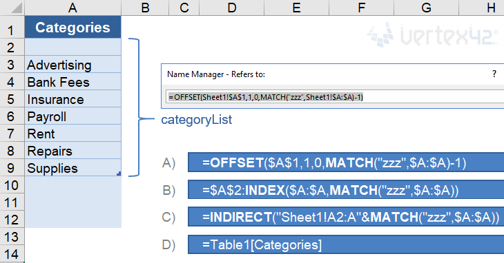
When we talk about a dynamic named range, we’re talking about using the Name Manager (via the Formula tab) to define a name for the formula, such as categoryList. We can then use that Name in other formulas or as the Source for drop-down lists.
This article isn’t about the awesome advantages of using Excel Names, though there are many. Instead, it is about the many different formulas you can use to create the dynamic named ranges.
To see these examples in action, download the Excel file below.
Download the Example File (DynamicRanges.xlsx)
Do you have a Dynamic Named Range challenge you need to solve? If you can’t figure it out after reading this article, go ahead and ask your question by commenting below.
This Page (contents):
- A) The OFFSET Function
- B) The INDEX Function for a Non-Volatile Dynamic Range
- C) The INDIRECT Function
- D) Structured References with Excel Tables
- E) The CHOOSE and IF Functions
- Find the Position of the LAST Value in the Column
- Bonus: Create a Dynamic Print Area
- No Dynamic Named Ranges in Google Sheets
Watch the Video
A) The OFFSET Function
The most common function used to create a dynamic named range is probably the OFFSET function. It allows you to define a range with a specific number of rows and columns, starting from a reference cell. The syntax for the OFFSET function is:
=OFFSET(reference,offset_rows,offset_cols,[height],[width])
The offset_rows and offset_cols values tell the function where you want the upper-left cell of your range to be, relative to the reference cell. The height and width values tell the function how many rows and columns you want to include in your range.
A Basic Customizable List
In the meal planner template, I have a list of meals that I use as the Source for many different drop-down lists. I want to allow the user to edit and add to the list, so the dynamic named range used by the drop-down needs to extend to the last value in the list. I could define the range as $A:$A (the entire column) or $A1:$A1000 (assuming they won’t add more than 1000 items to the list), but then I’d end up with a bunch of blank cells at the end of my drop-down list.
Using the OFFSET function, I define a range that starts at cell $A$1 and ends at the cell containing the last value in the column. If the last value in the column was on row 15, the formula for the named range would be:
=OFFSET($A$1,0,0,15,1)
To make this formula dynamic, I’ll use a formula or reference in place of the height value (15) to specify how many rows I want the range to include. I expect only text values in this list, so I’ll use the MATCH function to find the last text value in the column like this:
=OFFSET($A$1,0,0,MATCH("zzzz",$A:$A),1)
There are many formulas you can use to determine the height or width of the range, such as COUNTA, COUNT, VLOOKUP, LOOKUP, MATCH or various array formulas. What formula you use may depend on whether you expect there to be blank cells in the list, error values (like #N/A or #DIV/0!), or data of different types (text or numeric or both), and whether calculation speed is an issue.
Later in this article I’ll talk more about the various formulas for finding the last value in the range. For now, we’ll continue using MATCH.
A Robust Dynamic Range
When you allow a user to edit a list, they may end up deleting the first row in the list, or they might insert a row above the first row in the list (between the label row and the first item). To create a formula that works in spite of these actions by the user, I like to use a label for the reference and include the label in the range, as shown in the following examples.
Example 1: Include the label in the list
=OFFSET(reference,0,0,MATCH("zzz",range),1)
Example 2: Exclude the label from the list
=OFFSET(reference,1,0,MATCH("zzz",range)-1,1)
Notice in the second example that reference and range have not changed. To exclude the label from the list, we are using an offset of 1 row and subtracting one row from the number returned by the MATCH function.
B) The INDEX Function for a Non-Volatile Dynamic Range
A volatile function within a cell or named range is recalculated every time any cell in the worksheet recalculates (instead of just when one of the function’s arguments changes). Also, any formula that depends on a cell containing a volatile function is also recalculated. If you have a large file with thousands of inefficient formulas that reference a cell containing a volatile function, Excel may seem to take forever to recalculate. OFFSET is a volatile function. INDEX is not, so some people prefer to use INDEX for dynamic ranges.
The INDEX function can return the reference to a range or cell instead of just the value. That means that just like OFFSET, you can use INDEX in many places where Excel is expecting a cell reference. For example, to create the range A1:A4 you can use INDEX(A:A,1):INDEX(A:A,4).
We can use INDEX to create the same dynamic ranges shown in the OFFSET examples:
Example 1: Include the label in the list
=INDEX(range,1):INDEX(range,MATCH("zzz",range))
Example 2: Exclude the label from the list
=INDEX(range,2):INDEX(range,MATCH("zzz",range))
To exclude the label (the first cell in the range), the only change we needed to make was the «2» in INDEX(range,2). Using INDEX(range,1) and INDEX(range,2) instead of just a cell reference makes the formula more robust. It prevents the problem of having the reference changed to #REF! if the reference row gets deleted.
NOTEWhen using INDEX, the formulas cannot be entered directly as the Source for a drop-down list. But, if you create the formula as a dynamic named range, you can use the name as the Source for the drop-down list.
By the way, I learned about using the INDEX function to make a non-volatile dynamic range from Mynda Treacy at MyOnlineTrainingHub.com and Debra Dalgleish at Contextures.com.
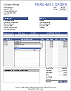 Purchase Order with Price List
See Dynamic Named Ranges in action. This template uses multiple customizable lists for selecting items descriptions, vendor and ship to addresses, and other options. The item description list uses the OFFSET formula and the other lists use the INDEX formula.
C) The INDIRECT Function
The INDIRECT function is another awesome function for creating dynamic ranges. It is also a volatile function, but like I mentioned above, that might not matter. The INDIRECT function lets you define a reference from a text string, and you can use concatenation to create the text string, like this:
=INDIRECT("Sheet1!A1:A"&row_num)
In the example shown at the top of this post, to create the reference «Sheet1!A2:A9» we replace row_num with MATCH(«zzz»,$A:$A) to return the row number of the last text value.
Important: When using INDIRECT to reference a range on a different worksheet, don’t forget to include the worksheet name in the string. When you enter a reference in the Refers To field via the Name Manager, Excel will automatically change $A:$A to «Sheet1!$A:$A» but it won’t know how to change your text string. This is one of the cons to using INDIRECT because if you change the name of the worksheet, you’ll need to remember to update your INDIRECT formula.
D) Structured References with Excel Tables
Beginning with Excel 2007, Microsoft introduced a new way to work with data in what are called Excel Tables, not to be confused with Data Tables, or other generic uses of the term table (yes, it is confusing).
If you use an official «Excel Table,» you can use a type of reference known as a structured reference. The structured reference uses the table name and the column labels like this:
=Table1[Categories]
You don’t need to know how to type the correct structured reference. While you are entering a formula, if you select the column in the Table, Excel will automatically change your reference to the structured reference.
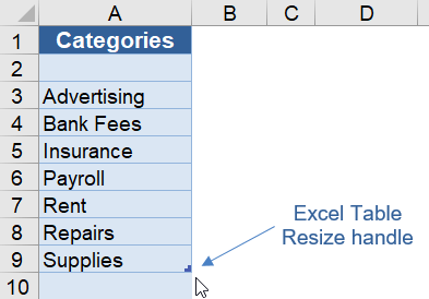
The reason these types of references can be considered dynamic is because of the unique way that table references behave when you expand or contract the table. Meaning, if you extend the table down by dragging the resize handle in the lower-right corner of the table, the reference =Table1[Categories] will automatically include the new rows.
So, instead of using an OFFSET formula to extend a range to the last value in a customizable list, we can let the user change the size of the list using the drag handle. Of course, this requires the user to know how to use Tables and the drag handle. That is one of the reasons I don’t often use this technique in my templates (that, and lack of compatibility with OpenOffice and Google Sheets).
E) The CHOOSE and IF Functions
Although I don’t use the CHOOSE function or nested IF formulas to create lists of variable length, they are pretty powerful functions for creating other types of dynamic ranges. For example, the two formulas below both return a different range (range_1, range_2 or range_3) based on a given number:
=CHOOSE(number,range_1,range_2,range_3,...)
=IF(number=1,range_1,IF(number=2,range_2,IF(number=3,range_3)))
The CHOOSE function is basically a shortcut for the nested IF formula in this case. When possible, I prefer using CHOOSE over nested IF formulas (if only to avoid having a million closing parentheses at the end of the formula ))))))))))).
See CHOOSE in action: My article «Create a Drop Down List in Excel» shows an example using CHOOSE to create a dependent drop down list.
Find the Position of the LAST Value in the Column
When using a dynamic named range for lists of variable length, we need to know how to find the numeric position of the last value in the column. In the examples above we used MATCH(«zzz»,range) for text values, but for numeric data or a combination of text and numeric data we may need to use something different. The formulas below cover all the scenarios I’ve come across.
The following image will be used for the example. It shows the reference and range and the position numbers of the values in the range.

1. Find the Position of the Last Numeric Value
The following formulas will allow the range to include blanks, error values, and text values, but the formulas will only return the position of the last numeric value. The result would be 4 in the example above.
=MATCH(1E+100,range,1)
=LOOKUP(42,1/ISNUMBER(range),ROW(range)-ROW(reference)+1)
See my article about VLOOKUP and INDEX-MATCH for a more detailed explanation of these MATCH and LOOKUP formulas. LOOKUP does not behave the same way in OpenOffice and Google Sheets. So, for maximum compatibility, I still prefer to use MATCH.
The value 9.99999999999999E+307 could be used for the MATCH function because it is the largest numeric value that can be stored in a cell, but that is kind of overkill. I prefer to use something more concise like 1E+100 or 10^100 (a googol).
2. Find the Position of the Last Text Value
The following formulas will allow the range to include blanks, error values, and numeric values, but the formulas will only return the position of the last text value (row 5 in the example above).
=MATCH("zzzz",range,1)
=LOOKUP(42,1/ISTEXT(range),ROW(range)-ROW(reference)+1)
Note: Using «zzzz» for the lookup value is not fool proof. The Greek, Cyrillic, Hebrew, and Arabic Unicode characters (and possibly other Unicode characters) come after z in the sort order. You might try using a high-value unicode symbol such as 🗿 if you expect the list to contain symbols.
3. Find the Position of the Last Non-Blank Value
When we want to return the last non-blank value, we can use the largest position returned by the two MATCH formulas listed above, or we can use the LOOKUP formula.
=MAX(MATCH(9E+307,range),MATCH("🗿",range))
=LOOKUP(42, 1/NOT(ISBLANK(range)), ROW(range)-ROW(reference)+1 )
Note that the empty string «» is not blank. It is treated as a text value.
A cell containing a formula is not blank, even if the formula returns an empty string. So, use the next method if you want to find the last non-empty value when you are using formulas that might return an empty string.
4. Find the Position of the Last Non-Empty Value «»
In many practical applications (like loan calculators), we may not necessarily want to find the last non-blank cell ( meaning no values or formulas), but instead may want to find the last non-empty cell.
If we define «empty» as the empty string «», then we can return the last non-empty value using the formula below. This might look like an array formula, but it isn’t, thanks to the way LOOKUP works (See this article on exceljet.net).
=LOOKUP(42, 1/(range<>""), ROW(range)-ROW(reference)+1 )
As I mentioned before, LOOKUP does not work the same way in OpenOffice and Google Sheets, but SUMPRODUCT provides a good solution.
=SUMPRODUCT(MAX((range<>"")*(ROW(range)-ROW(reference)+1)))
The SUMPRODUCT function allows you to avoid entering the formula as an array formula (not having to use Ctrl+Shift+Enter). Inside the SUMPRODUCT function, we are multiplying the boolean (FALSE=0 or TRUE=1) result for the (range<>»») comparison by the relative row number, so that the maximum result is the row number of the last blank cell.
Bonus: Create a Dynamic Print Area
When you create a print area in Excel via Page Layout > Print Area > Set Print Area, Excel actually creates a special named range called Print_Area. You can then go to Formulas > Name Manager and edit that named range to use a formula like this:
=OFFSET(start_cell,0,0,rows,columns)
This is a technique I use in some financial templates like the Home Mortgage Calculator to limit the print area based on the length of the payment schedule.
The catch: If you edit the Page Layout (margins, scaling, etc.), the Print_Area reference is changed to a regular reference. I’m not sure why the formula is removed, but this is basically a bug in Excel that has yet to be resolved. To avoid recreating the formula, I typically copy the formula and paste it into a text editor so that I can easily recreate the dynamic print area after I’m done making changes to the page layout.
No Dynamic Named Ranges in Google Sheets
Perhaps things will change in the future, but as of my last update (Sep 28, 2017), you cannot create named formulas using the Named Ranges feature in Google Sheets. This means that although you can use a Named Range for a drop-down list, you can’t create a Dynamic Named Range using a formula in Google Sheets.
Ben Collins shows how you can use a cell to create a text string like «A1:A»&row_num, name the cell, and then use INDIRECT(theName) to get some of the function of a dynamic named range. Unfortunately, that still doesn’t work for drop-down lists, because you can’t use INDIRECT(theCell) as the Range for a drop-down list.
References Related to Dynamic Named Ranges
- Dynamic Named Ranges at ozgrid.com — I think Dave Hawley’s site is the first place I saw the term «dynamic named range» used. Now, you can find articles on the subject at most Excel help sites.
- Using structured references with Excel tables at support.office.com
- Excel Named Ranges at contextures.com — A great article by Debra Dalgleish about how to create and use named ranges in Excel.
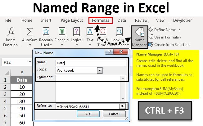
Excel Named Range (Table of Contents)
- Named Range in Excel
- Define Names from a Selected Range
- How to Create a Named Range in Excel?
Introduction to Named Range in Excel
Named Range just makes the process of working with formulas exciting, especially to keep track of things. It is just very convenient to assign a name to a range. If there is any change in that range, it becomes infinitely easier to update the range through the Name Manager. It totally allows us to bypass the process of manually updating every formula. Also, in cases of nested formulas, where one formula has to be used in another formula or maybe just used in a different location, all that needs to be done is to refer to the formula by its name.
The importance of named ranges is that one can use any names in the formula without worrying about the cell addresses/references. Any name can be assigned to a range. Any named constant or any data can be given a named range, and these names can be used instead of the actual formula. In this way, it becomes easier to understand the formulas. So, what this does is that it gives a range of cells in Excel a human-understandable name. By making use of named ranges, one can make the usage of formulas straightforward in Excel. One can give a name to a range in a formula or function, a constant, or a table. After starting to use names in a sheet, one can easily comprehend these names.
Define Names from a Selected Range
Firstly, one has to select the range that you want to give a name. Thereafter navigate to Formulas and then select Create from Selection.
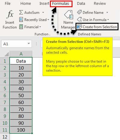
From the “Create Names from Selection” box, select either Bottom Row, Top Row, Left Column, or Right Column, and then click on OK.
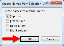
The cells are named based on labels in the designated range:
- First, use names in formulas and then focus on a cell and then enter a formula.
- The cursor has to be placed at the location where we want to use the named range in a formula.
- The name can be selected from the list that opens up after typing the name’s first letter.
- Alternatively, navigate to Formulas and then Use in Formula, followed by selecting the name that you intend to use.
- Press Enter.
It is also possible to update the named ranges from the Name Manager. The shortcut to update the named ranges from the Name Manager is Ctrl+F3. We just need to select the name that we wish to change and then proceed to change the reference directly.
How to Create Named Ranges in Excel?
Let us understand the concept of the Named Range through some examples.
You can download this Named Range Excel Template here – Named Range Excel Template
Example #1
Create a Named Range by using the Define Name option
- First, focus on the cells by selecting the range of cells.
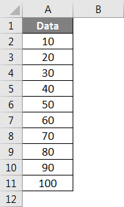
- Now, navigate to the Formulas tab. Next, go to the Defined Name group. Click to select Define Name.
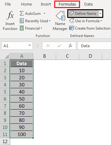
- Now once the New Name dialog box opens, mention three things -Name, Scope, Comment.
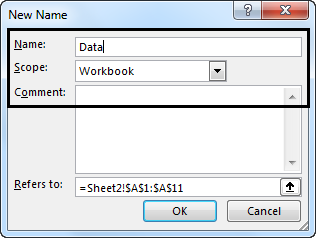
- Now in the “Name:” category, provide a name for the range.
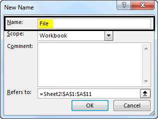
- Now in the “Scope:” category, from the dropdown, the name scope has to be set (by default, it is Workbook)
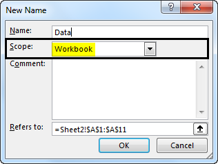
- Now move on to the ‘Refers to:’ section, verify the available reference, and modify it if required. After that, click on OK to save the changes you have made and close the dialog box.
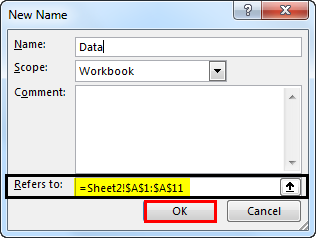
Example #2
Create a Named Range by utilizing the Name Manager
- Navigate to the Formulas tab and then proceed towards Define Name Group and then click on Name Manager.
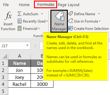
- Alternatively, you can also press Ctrl+F3, which is the shortcut for the same.

- Now, on the top, towards the Name Manager’s left corner, we have the ‘New’ button. Click on it.
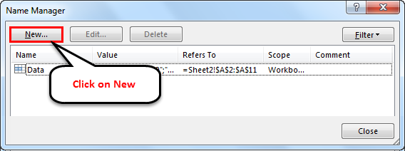
Then the New Name dialog box will open.
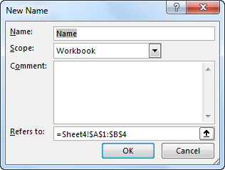
Example #3
Create a Named Range using VBA
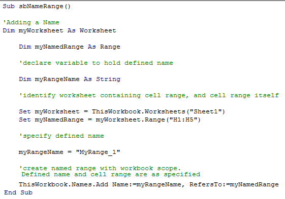
We can also create a Named Range in VBA.
So, this is what we did in the code snippet above:
- We created three variables – myWorksheet of Worksheet datatype, which will store the name of the Excel Worksheet, myNamedRange of Range datatype, which will hold the name of the range of cells that we wish to name, and myRangeName, of String datatype, which will hold the name of the Named Range.
- We defined our Worksheet (in the variable myWorksheet).
- We then went on to define the range of cells that we wanted to name (in the variable myNamedRange).
- After that, we defined the name of our Named Range in the variable myRangeName.
- After that, we proceed to create the Named Range and provide the reference to which it will point to.
This concludes the Named Range creation process through VBA.
Things to Remember
The following things must always be kept in mind while creating or dealing with Named Ranges in Excel.
- Named Ranges can have names that start with either a backslash (), letter, or underscore (_). Numbers or other special symbols are invalid as the starting character. If any other character other than letters, backslash or an underscore is given as the starting character, then Excel will throw an error.
- There is also a limitation on how long the name of a Named Range can be. The maximum length of a name can be 255 characters. Anything above 255 characters will cause Excel to throw an error.
- Every name has to be a continuous sequence of characters. There is no scope to have spaces, tabs, or any punctuation marks in the name. This is done so as to maintain uniformity and make the names easier.
- Another important instruction while working with Named Ranges is that a Named Range’s name must not have any conflict with cell references.
- As we saw, there is a limit on the maximum length for a name. Conversely, a name must also be of at least one character length at a minimum. Names are allowed to be of a single character length; however, there are few characters such as ‘r’ and ‘c’, which are reserved by Excel and can not be used as Names.
- As a bonus, Names aren’t case sensitive, which means that names such as “Jon”, “JON”, “jon” are all the same to Excel.
Recommended Articles
This has been a guide to Named Range in Excel. Here we discussed how to create a named range in excel along with practical examples and a downloadable excel template. You can also go through our other suggested articles to learn more –
- Excel Function for Range
- Range in Excel
- VBA Named Range
- VBA Range