
Name a cell
-
Select a cell.
-
In the Name Box, type a name.

-
Press Enter.
To reference this value in another table, type th equal sign (=) and the Name, then select Enter.
Define names from a selected range
-
Select the range you want to name, including the row or column labels.
-
Select Formulas > Create from Selection.
-
In the Create Names from Selection dialog box, designate the location that contains the labels by selecting the Top row, Left column, Bottom row, or Right column check box.
-
Select OK.
Excel names the cells based on the labels in the range you designated.
Use names in formulas
-
Select a cell and enter a formula.
-
Place the cursor where you want to use the name in that formula.
-
Type the first letter of the name, and select the name from the list that appears.
Or, select Formulas > Use in Formula and select the name you want to use.
-
Press Enter.
Manage names in your workbook with Name Manager
-
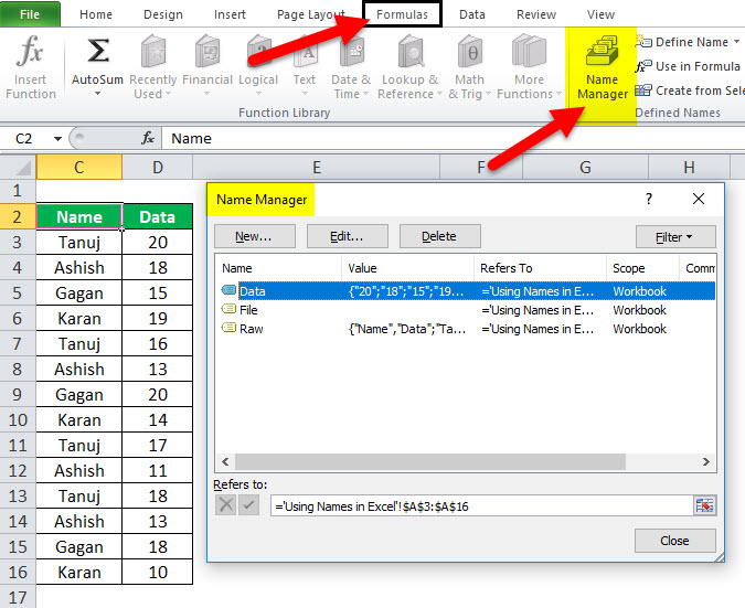
On the ribbon, go to Formulas > Name Manager. You can then create, edit, delete, and find all the names used in the workbook.
Name a cell
-
Select a cell.
-
In the Name Box, type a name.
-
Press Enter.
Define names from a selected range
-
Select the range you want to name, including the row or column labels.
-
Select Formulas > Create from Selection.
-
In the Create Names from Selection dialog box, designate the location that contains the labels by selecting the Top row,Left column, Bottom row, or Right column check box.
-
Select OK.
Excel names the cells based on the labels in the range you designated.
Use names in formulas
-
Select a cell and enter a formula.
-
Place the cursor where you want to use the name in that formula.
-
Type the first letter of the name, and select the name from the list that appears.
Or, select Formulas > Use in Formula and select the name you want to use.
-
Press Enter.
Manage names in your workbook with Name Manager
-
On the Ribbon, go to Formulas > Defined Names > Name Manager. You can then create, edit, delete, and find all the names used in the workbook.
In Excel for the web, you can use the named ranges you’ve defined in Excel for Windows or Mac. Select a name from the Name Box to go to the range’s location, or use the Named Range in a formula.
For now, creating a new Named Range in Excel for the web is not available.
Содержание
- Define and use names in formulas
- Name a cell
- Define names from a selected range
- Use names in formulas
- Manage names in your workbook with Name Manager
- Name a cell
- Define names from a selected range
- Use names in formulas
- Manage names in your workbook with Name Manager
- Need more help?
- Присвоение имени ячейкам Excel
- Присвоение наименования
- Способ 1: строка имен
- Способ 2: контекстное меню
- Способ 3: присвоение названия с помощью кнопки на ленте
- Способ 4: Диспетчер имен
- Excel Names and Named Ranges
- Excel Names — Introduction
- How to Name Cells
- Name Cells — Name Box
- Rules for Creating Names
- See Names on Worksheet
- Create List of Names on Worksheet
- What’s in the List?
- See Named Ranges by Zooming
- See Names in Name Manager
- Name Manager Dialog Box
- Delete an Excel Name
- Change a Named Range
- Create Names from Cell Text
- Create Names from Cell Text
- Notes on Creating Names from Cell Text
- Steps to Create Names from Cell Text
- One Location Selected
- Two Locations Selected
- All Four Locations Selected
- Create Name for a Value
- Frequently Used Values
- Special Values
- How to Use Excel Names
- Use Names for Quick Navigation
- Use Names in Formulas
- Name Box Tricks
- Resize the Name Box
- Select Cells
- Create a Dynamic Named Range
- Use a Named Excel Table
- First, create the table:
- Next, create a dynamic list of part IDs:
- Text the Dynamic Range
- Dynamic Named Range — Formula
- Dynamic Named Range Based on Formula
- Strange Characters Allowed in Excel Names
- More Fun with Excel Names
- In-Depth Excel Name Testing
- Get the Sample File
Define and use names in formulas
By using names, you can make your formulas much easier to understand and maintain. You can define a name for a cell range, function, constant, or table. Once you adopt the practice of using names in your workbook, you can easily update, audit, and manage these names.

Name a cell
In the Name Box, type a name.
To reference this value in another table, type th equal sign (=) and the Name, then select Enter.
Define names from a selected range
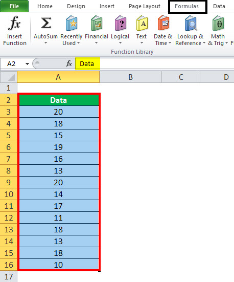
Select the range you want to name, including the row or column labels.
Select Formulas > Create from Selection.
In the Create Names from Selection dialog box, designate the location that contains the labels by selecting the Top row, Left column, Bottom row, or Right column check box.
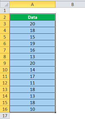
Excel names the cells based on the labels in the range you designated.
Use names in formulas
Select a cell and enter a formula.
Place the cursor where you want to use the name in that formula.
Type the first letter of the name, and select the name from the list that appears.
Or, select Formulas > Use in Formula and select the name you want to use.
Manage names in your workbook with Name Manager
On the ribbon, go to Formulas > Name Manager. You can then create, edit, delete, and find all the names used in the workbook.
Name a cell
In the Name Box, type a name.
Define names from a selected range
Select the range you want to name, including the row or column labels.
Select Formulas > Create from Selection.
In the Create Names from Selection dialog box, designate the location that contains the labels by selecting the Top row, Left column, Bottom row, or Right column check box.
Excel names the cells based on the labels in the range you designated.
Use names in formulas
Select a cell and enter a formula.
Place the cursor where you want to use the name in that formula.
Type the first letter of the name, and select the name from the list that appears.
Or, select Formulas > Use in Formula and select the name you want to use.
Manage names in your workbook with Name Manager
On the Ribbon, go to Formulas > Defined Names > Name Manager. You can then create, edit, delete, and find all the names used in the workbook.
In Excel for the web, you can use the named ranges you’ve defined in Excel for Windows or Mac. Select a name from the Name Box to go to the range’s location, or use the Named Range in a formula.
For now, creating a new Named Range in Excel for the web is not available.
Need more help?
You can always ask an expert in the Excel Tech Community or get support in the Answers community.
Источник
Присвоение имени ячейкам Excel

Для выполнения некоторых операций в Экселе требуется отдельно идентифицировать определенные ячейки или диапазоны. Это можно сделать путем присвоения названия. Таким образом, при его указании программа будет понимать, что речь идет о конкретной области на листе. Давайте выясним, какими способами можно выполнить данную процедуру в Excel.
Присвоение наименования
Присвоить наименование массиву или отдельной ячейке можно несколькими способами, как с помощью инструментов на ленте, так и используя контекстное меню. Оно должно соответствовать целому ряду требований:
- начинаться с буквы, с подчеркивания или со слеша, а не с цифры или другого символа;
- не содержать пробелов (вместо них можно использовать нижнее подчеркивание);
- не являться одновременно адресом ячейки или диапазона (то есть, названия типа «A1:B2» исключаются);
- иметь длину до 255 символов включительно;
- являться уникальным в данном документе (одни и те же буквы, написанные в верхнем и нижнем регистре, считаются идентичными).
Способ 1: строка имен
Проще и быстрее всего дать наименование ячейке или области, введя его в строку имен. Это поле расположено слева от строки формул.
- Выделяем ячейку или диапазон, над которым следует провести процедуру.
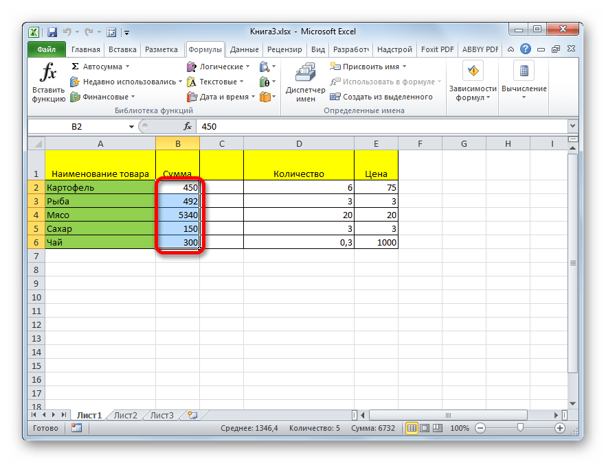
После этого название диапазону или ячейке будет присвоено. При их выделении оно отобразится в строке имен. Нужно отметить, что и при присвоении названий любым другим из тех способов, которые будут описаны ниже, наименование выделенного диапазона также будет отображаться в этой строке.
Способ 2: контекстное меню
Довольно распространенным способом присвоить наименование ячейкам является использование контекстного меню.
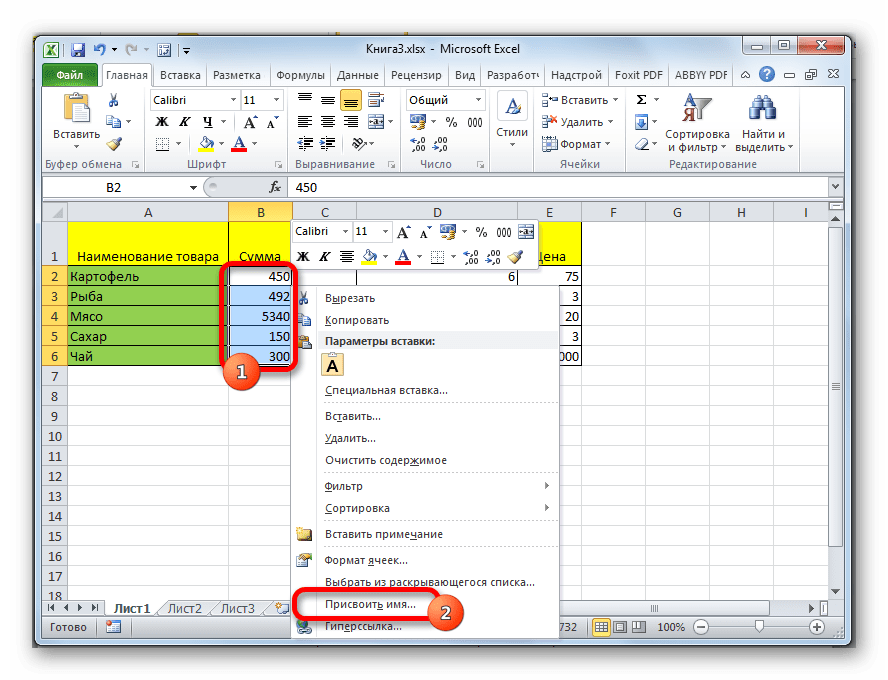
- Выделяем область, над которой желаем произвести операцию. Кликаем по ней правой кнопкой мыши. В появившемся контекстном меню выбираем пункт «Присвоить имя…».
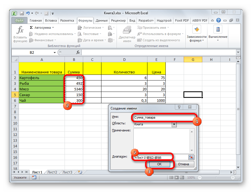
- Открывается небольшое окошко. В поле «Имя» нужно вбить с клавиатуры желаемое наименование.
В поле «Область» указывается та область, в которой при ссылке на присвоенное название будет идентифицироваться именно выделенный диапазон ячеек. В её качестве может выступать, как книга в целом, так и её отдельные листы. В большинстве случаев рекомендуется оставить эту настройку по умолчанию. Таким образом, в качестве области ссылок будет выступать вся книга.
В поле «Примечание» можно указать любую заметку, характеризующую выделенный диапазон, но это не обязательный параметр.
В поле «Диапазон» указываются координаты области, которой мы даем имя. Автоматически сюда заносится адрес того диапазона, который был первоначально выделен.
После того, как все настройки указаны, жмем на кнопку «OK».

Название выбранному массиву присвоено.
Способ 3: присвоение названия с помощью кнопки на ленте
Также название диапазону можно присвоить с помощью специальной кнопки на ленте.

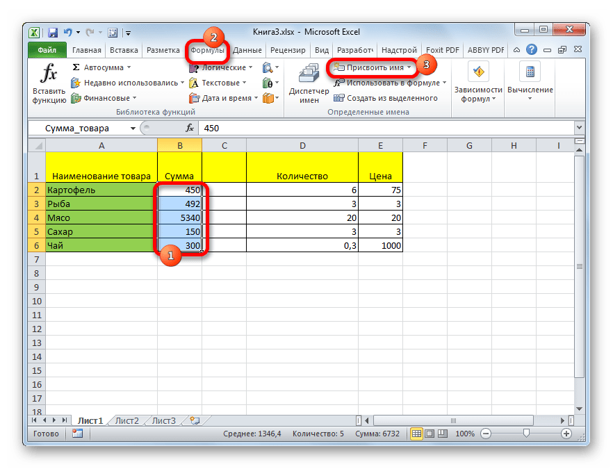
- Выделяем ячейку или диапазон, которым нужно дать наименование. Переходим во вкладку «Формулы». Кликаем по кнопке «Присвоить имя». Она расположена на ленте в блоке инструментов «Определенные имена».
- После этого открывается уже знакомое нам окошко присвоения названия. Все дальнейшие действия в точности повторяют те, которые применялись при выполнении данной операции первым способом.
Способ 4: Диспетчер имен
Название для ячейки можно создать и через Диспетчер имен.
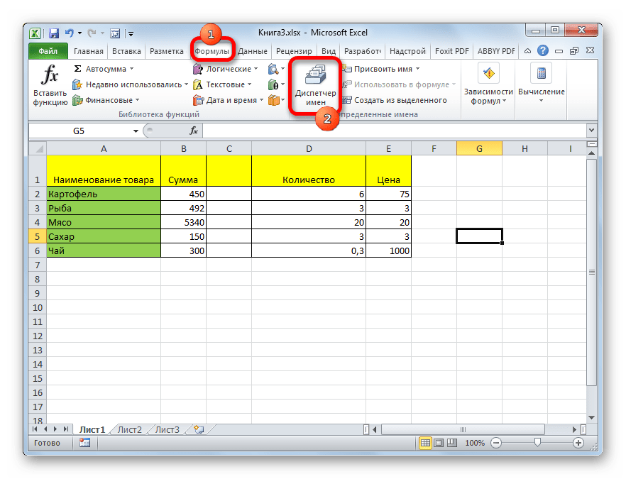
- Находясь во вкладке «Формулы», кликаем по кнопке «Диспетчер имен», которая расположена на ленте в группе инструментов «Определенные имена».
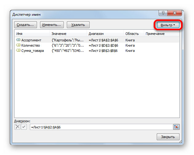
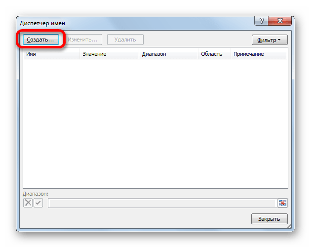
- Открывается окно «Диспетчера имен…». Для добавления нового наименования области жмем на кнопку «Создать…».
- Открывается уже хорошо нам знакомое окно добавления имени. Наименование добавляем так же, как и в ранее описанных вариантах. Чтобы указать координаты объекта, ставим курсор в поле «Диапазон», а затем прямо на листе выделяем область, которую нужно назвать. После этого жмем на кнопку «OK».
На этом процедура закончена.
Но это не единственная возможность Диспетчера имен. Этот инструмент может не только создавать наименования, но и управлять или удалять их.
Для редактирования после открытия окна Диспетчера имен, выделяем нужную запись (если именованных областей в документе несколько) и жмем на кнопку «Изменить…».

После этого открывается все то же окно добавления названия, в котором можно изменить наименование области или адрес диапазона.
Для удаления записи выделяем элемент и жмем на кнопку «Удалить».

После этого открывается небольшое окошко, которое просит подтвердить удаление. Жмем на кнопку «OK».

Кроме того, в Диспетчере имен есть фильтр. Он предназначен для отбора записей и сортировки. Особенно этого удобно, когда именованных областей очень много.
Как видим, Эксель предлагает сразу несколько вариантов присвоения имени. Кроме выполнения процедуры через специальную строку, все из них предусматривают работу с окном создания названия. Кроме того, с помощью Диспетчера имен наименования можно редактировать и удалять.
Источник
Excel Names and Named Ranges
Create Excel names that refer to cells, a constant value, or a formula. Use names in formulas, or quickly select a named range. Have fun with names too, and add strange characters, like a happy face!
Excel Names — Introduction
In Microsoft Excel, you can create names that refer to:
- Cell(s) on the worksheet
- Specific value
- Formula
After you define Excel names, you can:
- Use those names in a formula, instead of using a constant value or cell references.
- Type a name, to quickly go to that named range of cells
- Use the names as a source for the items in a data validation drop down list
The instructions below show how to create names and use names in your Excel files. Get the sample Excel workbook, to follow along with the instructions.
NOTE: To create a quick list of all the names in a workbook, see the Quick List of Names — No Macro instructions.
How to Name Cells
Watch this short video to see how to name a group of cells. Then, go to that named group of cells, or use the name in a formula. The written instructions are below the video. TOP
Name Cells — Name Box
You quickly name the selected cells by typing in the Name Box. NOTE: There are a few rules for Excel names, shown in the section below.
- Select the cell(s) to be named
- Click in the Name box, to the left of the formula bar
- Type a valid one-word name for the list, e.g. FruitList.
- Press the Enter key.

Rules for Creating Names
There are rules for Excel names on the Microsoft site, and I have briefly summarized those rules below.
However, despite these strict rules, some unusual characters are allowed in Excel names. There ahe examples of what is allowed, in the Strange Characters in Excel Names section, further donw on this page..
- The first character of a name must be one of the following characters:
- letter
- underscore (_)
- backslash ().
- Remaining characters in the name can be
- letters
- numbers
- periods
- underscore characters
- The following are not allowed:
- Space characters are not allowed as part of a name.
- Names can’t look like cell addresses, such as A$35 or R2D2
- C, c, R, r — can’t be used as names — Excel uses them as selection shortcuts
- Names are not case sensitive. For example, North and NORTH are treated as the same name.
See Names on Worksheet
The best way to see all the names that you’ve created is by using the Name Manager. The steps for that are in the next section, below.
However, there are 2 ways that you can also see the names on the worksheet:
Create List of Names on Worksheet
You can create a list of names on a worksheet, with a few easy steps. This is a quick way to double-check the names in the Excel file, and to see their Refers To formulas

To create the list, follow these steps:
- Insert a new worksheet, or select a cell in a blank area of an existing worksheet.
- On the Excel Ribbon, click the Formulas tab.
- In the Defined Names group, click Use in Formula
- At the bottom of the list of names, click Paste Names
- In the Paste Name dialog box, click Paste List
A 2-column list of names will be inserted, starting in the selected cell, so make sure you have room for your list
What’s in the List?
The list of names will contain all the workbook level names, unless there’s a duplicate sheet level name on the sheet where the name list is pasted.
In that case, the sheet level name appears in the list, instead of the workbook level name.
See Named Ranges by Zooming
To see some of the named ranges on a worksheet, use this quick trick:
- At the bottom right of the Excel window, click the Zoom Level setting
- In the Zoom dialog box, select Custom
- Type 39 in the percentage box, and click OK

The names of some ranges will appear on the worksheet, in blue text, like the MonthList in this screen shot.
- Names created with a formula, like YearList, won’t appear.
- Some ranges might be too small to show their name

See Names in Name Manager
To see details on all the names in the entire workbook, use the built-in Excel Name Manager tool.
To open the Name Manager, follow these steps
- On the Ribbon, click the Formulas tab
- In the Defined Names group, click Name Manager
OR, open the Name Manager with the keyboard shortcut Ctrl + F3
Name Manager Dialog Box
The Name Manager dialog box opens, showing a list of workbook level and worksheet level names.
- In the list, click on the name that you want to see details for
- At the bottom, the Refers To box shows the location of that named range, or a formula, if the name is not a range of cells
Delete an Excel Name
After you create a named range, you might need to delete that Excel name later. Sometimes, a name is no longer needed in a workbook.
Follow these steps to delete a name in Excel:
- On the Excel Ribbon, click the Formulas tab
- Click Name Manager
- In the list, click on the name that you want to delete
- At the top of the Name Manager, click the Delete button.
- A confirmation message appears, asking «Are you sure you want to delete the name ___?»
- To delete the name, click the OK button, or click the Cancel button, if you change your mind.
- Click Close, to close the Name Manager
Change a Named Range
After you create a named range, you might need to change the cells that it refers to. This short video shows the steps, and there are written steps below the video.
Follow these steps to change the range reference:
- On the Ribbon, click the Formulas tab
- Click Name Manager
- In the list, click on the name that you want to change
- In the Refers To box, change the range reference, or drag on the worksheet, to select the new range.
- Click the check mark, to save the change
- Click Close, to close the Name Manager TOP

Create Names from Cell Text
To quickly name individual cells, or individual ranges, you can use heading cell text as the names. Watch this video to see the steps. Written instructions are below the video.
Create Names from Cell Text
A quick way to create names is to base them on heading cell text (worksheet labels). In the example shown below, the cells in column E will be named, based on the labels in column D.

Notes on Creating Names from Cell Text
The cell text might be altered slightly, when the name is created. For example:
- If the labels contains space characters, those spaces are replaced with an underscore.
- Other invalid characters, such as & (ampersand) and # (number sign) will be removed, or replaced by an underscore character.
For more information on invalid characters, see the section above — Rules for Excel Names
Steps to Create Names from Cell Text
To name cells, or ranges, based on worksheet labels, follow these steps:
- Select the labels and the cells that are to be named.
- The labels can be above, below, left or right of the cells to be named.
- In this example, the labels are in column B, to the left of the cells that will be named.

- On the Excel Ribbon, click the Formulas tab
- Then, in the Defined Names group, click Create from Selection.

In the Create Names From Selection window, there is is heading, «Create Names From Values in the»
Below that heading, there 4 check boxes:
- Top Row
- Left Column
- Bottom Row
- Right Column
To create the names:
- In the dialog box, add a check mark to one or more of the cell locations, so the name will use text from those cells.
- Click the OK button, to create the names
One Location Selected
For example, in the screen shot below:
- label text is in the left column of the selected cells.
- Left column option has a check mark
 Five names will be created: Full_Name, Street, City, Province, Postal_Code
Click on a cell to see its name.
- In the screen shot below, cell C4 is selected, and you can see its name in the Name Box — Full_Name.
- The space character was replaced with an underscore.
Two Locations Selected
For the next example, in the screen shot below, two locations are selected:
When multiple locations are selected for the cell text, names are created for each selected location.
In the example shown below, 4 names will be created:

All Four Locations Selected
For the next example, in the screen shot below, all four of the locations are selected:
- Top Row
- Left column
- Bottom Row
- Right column
A name is created for all 8 of the label text cells:
- North, South, City, Stores, Old, New, Market Count
 Each named range includes the non-label cells adjacent to it. For example, both the City name and the Market name refer to the same two cells

Create Name for a Value
Most Excel names refer to ranges on the worksheet, but names can also be used to store a value.
Frequently Used Values
For example, create a name to store a percentage amount that you use frequently, such as a retail tax rate:
- Name: TaxRate
- Refers To: =0.5
Then, use that name in formulas, instead of typing in the value

Special Values
You can also create names to store values that are difficult to enter. For example, some formulas use this strange-looking number. According to Excel specifications on the Microsoft site, that is the largest positive number that you can type into an Excel cell.
- 9.99999999999999E+307
Instead of typing that number into your formulas, you could define a name, using that value (copy the number from this page before you create the name):
- Name: XL_Max
- Refers To: 9.99999999999999E+307

Then, use the XL_Max name in formulas, like this LOOKUP formula that finds the last number in a column.
=LOOKUP(9.99999999999999E+307, WeightData[Wt])

How to Use Excel Names
After creating names, you can use them:
Use Names for Quick Navigation
If a name refers to a range, you can select that name in the Name Box dropdown list, to select the named range on the worksheet.
NOTE: If a name does not appear in the drop down list, you can type the name instead

Use Names in Formulas
You can also use names in formulas. For example, you could have a group of cells with quantities sold. Name those cells Quantity, then use this formula to calculate the total amount:

Name Box Tricks
In addition to using the Name Box to create a named range, or to select a named range, here are a few other Name Box tricks.
Resize the Name Box
In old versions of Excel, the Name Box was a set width, and you couldn’t change that. Here’s how you can adjust the Name Box width in newer versions:
- Point to the 3-dot button at the right side of the Name Box
- When the pointer changes to a 2-headed arrow, drag left or right, to change the width

Select Cells
Another handy trick is that you can use the Name Box to select unnamed cells too. Here are a couple of ways that trick can be useful — unhide columns, or fill a long range of cells.
Here’s a quick way to unhide specific columns, and leave others hidden.
With Excel’s AutoFill feature, you can create a list of dates, or numbers, or other sequences, very quickly. Just type one or two values as the starting sequence, select those cells, and double-click the Fill Handle to fill down to the last row of data.
Sometimes though, there’s no data in the adjacent column, so AutoFill won’t work with a double-click. You could drag the Fill Handle down, but that’s not very efficient if you need to create a long series.
Here’s how to create a list of 1000 numbers in column A:
- Click in the Name Box
- Type a1:a1000 in the Name Box, and press Enter
- With the cells selected, type the number 1, and press Ctrl+Enter
- Next, select cell A1, and type the 1st number in your series, e.g. 5
- Select cell A2, and type the 2nd number in your series, e.g. 10
- Select cells A1 and A2, and double-click the Fill Handle, to create the series of 1000 numbers

Create a Dynamic Named Range
If the list that you want to name will change frequently, having items added and removed, you should create a dynamic named range. A dynamic named range will automatically adjust in size, when the list changes. Here are two ways to create a dynamic named range:
Use a Named Excel Table
The easiest way to create a dynamic named range is to start by creating a named Excel table. Then, define a range based on one or more columns in that table.
In this example there is a list of parts on the worksheet, and a named table, and dynamic named ranges will be created. Later, if you add new items to the table, the named range will automatically expand.
First, create the table:
- Select a cell in the parts list
- On the Ribbon’s Insert tab, click Table
- Check that the correct range has been selected, and add a check mark to My Table Has Headers
- Click OK, to create the table.

(optional) Change the table’s default name (e.g. Table1) to a meaningful name, such as tblParts

Next, create a dynamic list of part IDs:
- Select cells A2:A9, which contain the Part IDs (not the heading)
- Click in the Formula Bar, and type a one-word name for the range: PartIDList
- Press the Enter key, to complete the name.

To see the name’s definition, follow these steps:
- Click the Ribbon’s Formulas tab, and click Name Manager.
- There are two named items in the list:
- the Parts table, with the default name, Table1 (or the name that you gave to the table)
- the PartIDList, which is based on the PartID field in Table1.

Text the Dynamic Range
Because the PartIDList named range is based on a named table, the list will automatically adjust in size if you add or remove part IDs in the list.
- Add a new item in the list of Part IDs
- In the Name Box, select the PartIDList name
- The named range is selected, and it includes the new Part ID. TOP

Dynamic Named Range — Formula
When you create a named range in Excel, it doesn’t automatically include new items. If you plan to add new items to a list, you can use a dynamic formula to define an Excel named range. Then, as new items are added to the list, the named range will automatically expand to include them.
The written instructions are below the video.
Dynamic Named Range Based on Formula
If you don’t want to use a named table, you can use a dynamic formula to define a named range. As new items are added, the range will automatically expand.
Note: Dynamic named ranges will not appear in the Name Box dropdown list. However, you can type the names in the Name Box, to select that range on the worksheet.
- On the Ribbon, click the Formulas tab
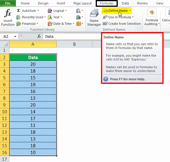
- Click Define Name
- Type a name for the range, e.g. NameList
- Leave the Scope set to Workbook.

=OFFSET(Sheet1!$A$1,0,0,COUNTA(Sheet1!$A:$A),1)
In this example, the list is on Sheet1, starting in cell A1
The arguments used in this Offset function are:
- Reference cell: Sheet1!$A$1
- Rows to offset: 0
- Columns to offset: 0
- Number of Rows: COUNTA(Sheet1!$A:$A)
- Number of Columns: 1
- Note: for a dynamic number of columns, replace the 1 with:
COUNTA(Sheet1!$1:$1)
Strange Characters Allowed in Excel Names
Even though Microsoft’s rules for Excel names say that you must use only letters, numbers, periods, underscores and backslashes, other characters are allowed.
Based on testing, «letters» has a broad interpretation, and goes well beyond the basic letters of the alphabet. You can use a wide variety of Unicode characters too!
For example, the screen shot below shows Excel names created by Peter B. He used Unicode text in his Excel names (shown below), to create arrows and subscript in Excel names, for a statistics workbook.

More Fun with Excel Names
Inspired by Peter’s examples, I did a few simple name tests, using characters created with the Alt key and Number keypad. For example:
- In the Name Box, I typed the lower-case letter “a” , then Alt+1, Alt+30 and Alt+31 (use the number keypad), The Alt key combonations created a happy face, up arrow, and down arrow in the name
- In another test, Excel used characters from cell D2, when I created a name using the Create From Selection technique on that range.
- In the Name Manager, I created a couple of names with Unicode characters. The special characters showed up correctly in the Name Manager, but appear as question marks in the Name Box drop down list.
In the screen shot below, you can see the list of unconventional names that I created.

In-Depth Excel Name Testing
For an in-depth look at what characters are allowed in Excel names, see Martin Trummer’s GitHub project excel-names.
Martin has done an in-depth study of what’s allowed, beyond the basic letters and numbers. When you visit Martin’s GitHub page, you’ll find written examples, and an Excel file to download.
Here is a screen shot from Martin’s Excel file, with his test results.

Get the Sample File
To follow along with the instructions on this page, download the Excel Names Sample File. The zipped file is in xlsx format, and does not contain any macros. TOP
Источник
Содержание
- Присвоение наименования
- Способ 1: строка имен
- Способ 2: контекстное меню
- Способ 3: присвоение названия с помощью кнопки на ленте
- Способ 4: Диспетчер имен
- Вопросы и ответы
Для выполнения некоторых операций в Экселе требуется отдельно идентифицировать определенные ячейки или диапазоны. Это можно сделать путем присвоения названия. Таким образом, при его указании программа будет понимать, что речь идет о конкретной области на листе. Давайте выясним, какими способами можно выполнить данную процедуру в Excel.
Присвоение наименования
Присвоить наименование массиву или отдельной ячейке можно несколькими способами, как с помощью инструментов на ленте, так и используя контекстное меню. Оно должно соответствовать целому ряду требований:
- начинаться с буквы, с подчеркивания или со слеша, а не с цифры или другого символа;
- не содержать пробелов (вместо них можно использовать нижнее подчеркивание);
- не являться одновременно адресом ячейки или диапазона (то есть, названия типа «A1:B2» исключаются);
- иметь длину до 255 символов включительно;
- являться уникальным в данном документе (одни и те же буквы, написанные в верхнем и нижнем регистре, считаются идентичными).
Способ 1: строка имен
Проще и быстрее всего дать наименование ячейке или области, введя его в строку имен. Это поле расположено слева от строки формул.
- Выделяем ячейку или диапазон, над которым следует провести процедуру.
- В строку имен вписываем желаемое наименование области, учитывая правила написания названий. Жмем на кнопку Enter.

После этого название диапазону или ячейке будет присвоено. При их выделении оно отобразится в строке имен. Нужно отметить, что и при присвоении названий любым другим из тех способов, которые будут описаны ниже, наименование выделенного диапазона также будет отображаться в этой строке.
Способ 2: контекстное меню
Довольно распространенным способом присвоить наименование ячейкам является использование контекстного меню.
- Выделяем область, над которой желаем произвести операцию. Кликаем по ней правой кнопкой мыши. В появившемся контекстном меню выбираем пункт «Присвоить имя…».
- Открывается небольшое окошко. В поле «Имя» нужно вбить с клавиатуры желаемое наименование.
В поле «Область» указывается та область, в которой при ссылке на присвоенное название будет идентифицироваться именно выделенный диапазон ячеек. В её качестве может выступать, как книга в целом, так и её отдельные листы. В большинстве случаев рекомендуется оставить эту настройку по умолчанию. Таким образом, в качестве области ссылок будет выступать вся книга.
В поле «Примечание» можно указать любую заметку, характеризующую выделенный диапазон, но это не обязательный параметр.
В поле «Диапазон» указываются координаты области, которой мы даем имя. Автоматически сюда заносится адрес того диапазона, который был первоначально выделен.
После того, как все настройки указаны, жмем на кнопку «OK».
Название выбранному массиву присвоено.
Способ 3: присвоение названия с помощью кнопки на ленте
Также название диапазону можно присвоить с помощью специальной кнопки на ленте.
- Выделяем ячейку или диапазон, которым нужно дать наименование. Переходим во вкладку «Формулы». Кликаем по кнопке «Присвоить имя». Она расположена на ленте в блоке инструментов «Определенные имена».
- После этого открывается уже знакомое нам окошко присвоения названия. Все дальнейшие действия в точности повторяют те, которые применялись при выполнении данной операции первым способом.
Способ 4: Диспетчер имен
Название для ячейки можно создать и через Диспетчер имен.
- Находясь во вкладке «Формулы», кликаем по кнопке «Диспетчер имен», которая расположена на ленте в группе инструментов «Определенные имена».
- Открывается окно «Диспетчера имен…». Для добавления нового наименования области жмем на кнопку «Создать…».
- Открывается уже хорошо нам знакомое окно добавления имени. Наименование добавляем так же, как и в ранее описанных вариантах. Чтобы указать координаты объекта, ставим курсор в поле «Диапазон», а затем прямо на листе выделяем область, которую нужно назвать. После этого жмем на кнопку «OK».
На этом процедура закончена.
Но это не единственная возможность Диспетчера имен. Этот инструмент может не только создавать наименования, но и управлять или удалять их.
Для редактирования после открытия окна Диспетчера имен, выделяем нужную запись (если именованных областей в документе несколько) и жмем на кнопку «Изменить…».
После этого открывается все то же окно добавления названия, в котором можно изменить наименование области или адрес диапазона.
Для удаления записи выделяем элемент и жмем на кнопку «Удалить».
После этого открывается небольшое окошко, которое просит подтвердить удаление. Жмем на кнопку «OK».
Кроме того, в Диспетчере имен есть фильтр. Он предназначен для отбора записей и сортировки. Особенно этого удобно, когда именованных областей очень много.
Как видим, Эксель предлагает сразу несколько вариантов присвоения имени. Кроме выполнения процедуры через специальную строку, все из них предусматривают работу с окном создания названия. Кроме того, с помощью Диспетчера имен наименования можно редактировать и удалять.
Еще статьи по данной теме:
Помогла ли Вам статья?
Updated: 12/31/2020 by
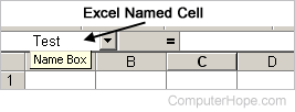
To create a named cell in Microsoft Excel, select the cell and click the Name Box next to the formula bar, as shown in the image. This bar has the current cell location printed in it. For example, if you’re in cell A1, it should currently say A1 in the Name Box. In the Name Box, type the name you want to name the cell and press Enter.
Once a cell is named, you can refer to this cell in a formula, chart, or anything else that uses cell references. For example, let’s assume you named a cell profits. When creating a new formula, you could type =sum(B10+profits) to add cell B10 plus the value in the profits cell.
Tip
When naming a cell or range, it can only be one word with no spaces.
Tip
In Excel, use the shortcut key Ctrl+F3 to open the Name Manager. In the Name Manager, you can create, edit, and delete any Excel names. Once a name is created, you can use the shortcut key F3 to insert any name.
Why is it beneficial to name cells in a spreadsheet?
It is easier to use the name of a cell instead of the cell reference. For example, it’s easier to remember «profits» (as mentioned earlier) instead of the cell containing the profits value.
 Excel is one of the applications included in Microsoft Office, Microsoft’s suite of office productivity software. Microsoft Office applications can run on almost every system businesses use, including Windows and Mac. Excel is specifically used for creating spreadsheets, basic databases, analyzing data, and even simplifying management. Many spreadsheets can be a challenge to navigate. One way to make your spreadsheets easier to get around is to name the cells.
Like other spreadsheet applications, Microsoft Excel documents are based on cells that can be arranged into rows and columns. It is within these cells that data is entered when creating a worksheet for various functions including data management and computations, etc. Each cell in the spreadsheet has a corresponding name, which is identified by its column letter and row number.
For instance, the cell under column A that belongs to row 1 has the default name A1. You will see this in the name box, which is located on the upper left side of the spreadsheet, next to the formula bar. This name can actually be changed however.
Why name cells in Excel
As mentioned, the default name for each cell in an Excel spreadsheet is based on the relevant column and row. One of the reasons why you may want to change this name is to make it easier to find what you are looking for, especially when there’s a lot of information in a particular spreadsheet. For instance, if you name a particular cell ‘Total’, searching for this word is much faster than scrolling through the spreadsheet to find the correct cell or trying to remember its specific column and row.
This is also the case when creating formulas for computations. Instead of using the cells’ column letter and row number, it’s more convenient to use a name that you can easily understand. For example, naming one cell ‘GrossIncome’ and the other one ‘Deductions’ makes it easier for you to compute net income by subtracting Deductions from GrossIncome for the result.
Another benefit of naming cells is that it is easier for other users to understand. If you are sharing the spreadsheet or workbook with other colleagues or business associates, using cell names that are easy for everyone to identify reduces potential confusion.
How to name cells in Excel
Naming cells in Excel can be done in two ways. The first is by changing the name directly on the name box and the other one is by defining names under the Formulas menu. The difference is that when naming a cell through the define name feature of the menu you can select its specific scope.
This determines where the specific name will be recognized as having the same value, such as in the entire workbook or in a specific spreadsheet only. Changing the name in the name box will automatically determine the workbook as its scope rather than the whole spreadsheet.
Changing a cell name in the name box:
- Select the cell that you want to name.
- Go to the name box and type the name you prefer.
- Hit enter on your keyboard.
Defining a cell name:
- Select the cell that you wish to name.
- Click the Formulas menu.
- Choose Define Name.
- Type the name of the cell in the new window that pops up.
- Select the Scope.
- Click OK.
Remember that a cell name should not contain any spaces. The uppercase and lowercase letters R and C are also not available as cell names, since they represent column and row. Furthermore, aside from letters, the first character of a cell name can also be a backslash or an underscore. The rest can be a combination of letters, underscores, periods and numbers, which can be up to 255 characters.
If you have further questions about changing the cell name in Excel, please don’t hesitate to give us a call.
In a Microsoft Excel worksheet, a cell can be given a name. And it is very EASY to name a cell: You click on the cell, put the cursor in the «Name Box» to the left of the Formula Bar, type a name, and press Enter. Then you can reference that cell by name in other parts of the workbook.

Also, when you click in a cell, if there is a cell name associated with that cell, it will display in the name box as shown in the worksheet image below.
In the example above we named the cell «Sub1» because we reference this Subtotal in a Summary worksheet.
However, after naming a cell, it seems like Excel won’t let you delete or change the name! Right? Because if you click in the Name Box and type over the name or delete the name, NOTHING HAPPENS! And Excel Help doesn’t seem to help.
So, how do I change or delete a cell name in an Excel spreadsheet? It’s pretty easy … it’s just hidden!
So open your Excel spreadsheet and follow the directions below.
1. Click the Formulas tab at the top of the worksheet. Then click Name Manager on the «Defined Names» section of the ribbon. The Name Manager window displays and lists ALL of the cell names that have ever been defined in the worksheets in that workbook.
2. Click on the cell name that you want to change, and click the Edit button. The Edit Name window displays.
3. Retype the name and click OK. When finished, click Close on the Name Manager window.
To Delete a Cell Name
1. Click the Formulas tab at the top of the worksheet. Then click Name Manager on the «Defined Names» section of the ribbon. The Name Manager window displays and lists ALL of the cell names that have ever been defined in the worksheets in that workbook.
2. Click on the cell name that you want to delete, and click Delete button.
3. Click OK on the «are you sure» popup and then click Close on the Name Manager window.
Whew! By the way, our main tutorial website has just had an exciting makeover! Besides our popular beginner’s tutorials such as Excel Math Basics: A Beginner’s Guide and Beginner’s Guide to Creating Charts in Excel, we’ve added tutorials on several more Excel functions, such as Nested IFs and Advanced Use of the COUNTIF Function.
Cheers!
What is Name Range in Excel?
The name range in Excel is the range that has been given a name for future reference. To make a range as a named range, select the range of data and then insert a table. Then, we put a name to the range from the Name Box on the left-hand side of the window. After this, we can refer to the range by its name in any formula.
The name range in Excel makes it much cooler to keep track of things, especially when using formulas. You can assign a name to a range. No problem with any change in that range; you need to update the range from the Name Manager in ExcelThe name manager in Excel is used to create, edit, and delete named ranges. For example, we sometimes use names instead of giving cell references. By using the name manager, we can create a new reference, edit it, or delete it.read more. You do not need to update every formula manually. Similarly, you can create a name for a formula. Then, if you want to use that formula in another formula or another location, refer to it by name.
- The name ranges are significant because you can put any names in your formulas without considering cell references/addresses. Furthermore, you can assign the range with any name.
- Create a named range for any data or a named constant and use these names in your formulas in place of data references. In this way, you can make your formulas easier to comprehend better. A named range is just a human-understandable name for a range of cells in Excel.
- Using the name range in Excel, you can simplify and comprehend your formulas better. For example, you can assign a name for a range in an excel sheet for a function, a constant, or table data. Once you start using the names in your Excel sheet, you can easily understand these names.
Table of contents
- What is Name Range in Excel?
- Define Names For a Selected Range
- Excel names the cells based on the labels in the range you designated.
- Update named ranges in the Name Manager (Control + F3)
- How to Use Name Range in Excel?
- Example #1 Create a name by using the Define Name option
- Example #2 Make a named range by using Excel Name Manager
- Name Range using VBA.
- Things to Remember
- Recommended Articles
- Define Names For a Selected Range
Define Names For a Selected Range
- Select the data range you want to assign a name, then select formulas and create from the selection.
- Click on the “Create Names from Selection,” then select the “Top row,” “Left column,” “Bottom row,” or “Right column” checkbox and select “OK.”
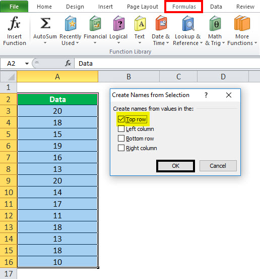
Excel names the cells based on the labels in the range you designated.
- Use names in formulas, then select a cell and enter a formula.
- Place the cursor where you want to use the name range formula.
- Type the first letter of the name, and select the name from the list that appears.
- Or, select “Formulas,” then use in formula and select the name you want to use.
- Press the “Enter” key.
Update named ranges in the Name Manager (Control + F3)
You can update the name from the Name Manager. Press “Ctrl” and “F3” to update the name. Select the name you want to change, then change the reference range directly.
How to Use Name Range in Excel?
Let us understand the working of conditional formatting by simple Excel examples.
You can download this Using Names in Excel Template here – Using Names in Excel Template
Example #1 Create a name by using the Define Name option
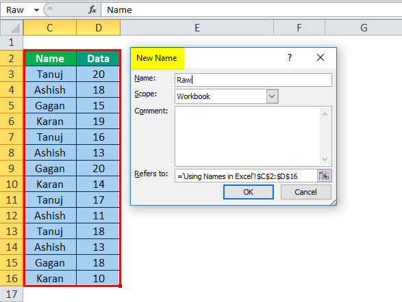
Below are the steps to create a name by using the “Define Name” option:
- First, select the cell(s).

- On the “Formulas” tab, click the “Define Name” in the “Defined Names” group.

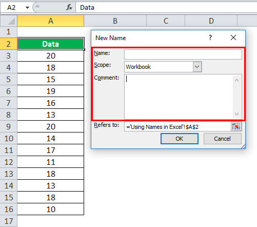
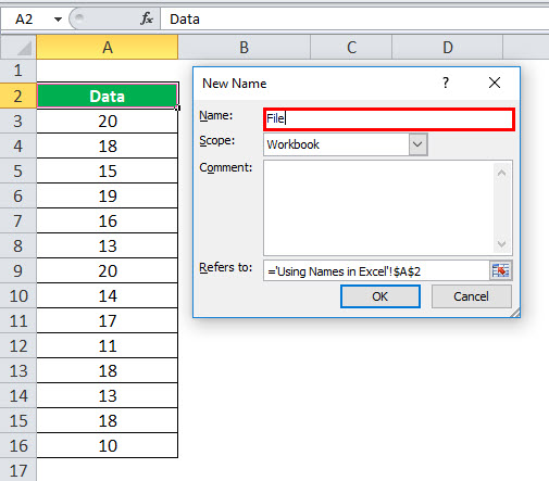
- In the “New Name” dialog box, specify three things:

- First, in the “Name” box, type the range name.

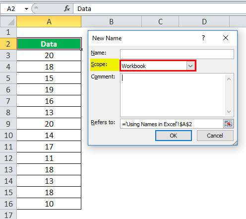
- In the “Scope” drop-down, set the name scope (Workbook by default).

- In the “Refers to” box, check the reference and correct it if needed. Finally, click “OK” to save the changes and close the dialog box.


Example #2 Make a named range by using Excel Name Manager
- Go to the “Formulas” tab, then the “Defined Names” group, and click the “Name Manager” or press “Ctrl + F3” (the preferred way).
- In the top left-hand corner of the “Name Manager” dialog window, click the “New… button:”
Name Range using VBA.
We can apply the naming in VBA; here is the example as follows:
Sub sbNameRange()
‘Adding a Name
Names.Add Name:=”myData”, RefersTo:=”=Sheet1!$A$1:$A$10″
‘OR
‘You can use Name property of a Range.
Sheet1.Range(“$A$1:$A$10”).Name = “myData”
End Sub
Things to Remember
We must follow the below instruction while using the name range.
- The names can start with a letter, backslash (), or an underscore (_).
- The name should be under 255 characters long.
- The names must be continuous and cannot contain spaces and most punctuation characters.
- There must be no conflict with cell references in names using in excelCell reference in excel is referring the other cells to a cell to use its values or properties. For instance, if we have data in cell A2 and want to use that in cell A1, use =A2 in cell A1, and this will copy the A2 value in A1.read more.
- We can use single letters as names, but the letters “r” and “c” are reserved in Excel.
- The names are not case-sensitive – “Tanuj”, “TANUJ”, and “TaNuJ” are all the same in Excel.
Recommended Articles
This article is a guide to the Name Range in Excel. We discuss using names in Excel, practical examples, and downloadable Excel templates here. You also may look at these useful functions in Excel: –
- VBA RangeRange is a property in VBA that helps specify a particular cell, a range of cells, a row, a column, or a three-dimensional range. In the context of the Excel worksheet, the VBA range object includes a single cell or multiple cells spread across various rows and columns.read more
- Data Tables ExcelA data table in excel is a type of what-if analysis tool that allows you to compare variables and see how they impact the result and overall data. It can be found under the data tab in the what-if analysis section.read more
- Data Validation using ExcelThe data validation in excel helps control the kind of input entered by a user in the worksheet.read more
- Paste SpecialPaste special in Excel allows you to paste partial aspects of the data copied. There are several ways to paste special in Excel, including right-clicking on the target cell and selecting paste special, or using a shortcut such as CTRL+ALT+V or ALT+E+S.read more