Excel multiple values in one cell to multiple cells

I am working with patent data and I have multiple values (International Patent Classifications) separated by a comma in one cell. For instance: C12N, C12P, A01 (within one cell). I would like to analyze how many different 4-digit classifications each patent has. To do so, I need to, first, separate the individual values and put each of them into an individual cell. Second, I need to count the unique values (each placed then in separate columns) for each row.

How can I separate the individual values within one cell into multiple cells within Excel or R. Is there any excel or R function you can suggest?

Here is reproducible example on how the data looks like in R or in Excel.

#Example of how the data looks like 
Publication_number<-c(12345,10012,23323,44556,77999)
IPC_class_4_digits<-c("C12N,CF01,C345","C12P,F12N,F039","A014562,F23N", "A01C, A01B, A01F, A01K, A01G", "C10N, C10R, C10Q, C12F")

data_example<-cbind(Publication_number, IPC_class_4_digits)
View(data_example)

The expected about should be a column «counts» counting the number of different 4-digit numbers. In this case => c(3, 3, 2, 5, 4)

This post will explain that how to split a cell into two or more cells within a single column. How do I convert one cell to multiple cells or rows in Excel. How to split the contents of a cell into multiple adjacent cells in with Text to Columns feature or with VBA code in Excel.

For examples, you want to split the text string of text in one single cell B1 into multiple rows in one single columns C. just do the following tutorial.

Split One Cell into Multiple Cells with Text to Columns Feature

#1 Select the Cell B1 that contains the text you want to split.

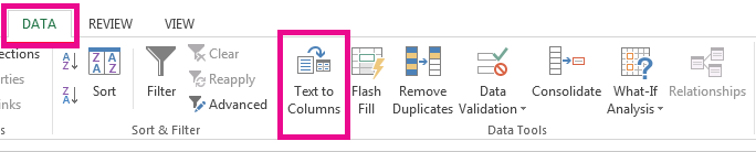
#2 go to Data tab, click Text to Columns command under Data Tools group.

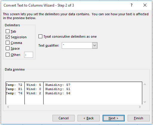
#3 the Convert Text to Columns Wizard window will appear. Choose Delimited if it is not already selected, and then click Next button.

#4 select the delimiter or delimiters to define the places where you want to split the cell content. Check Semicolon, and clear the rest of the boxes under Delimiters section. Or check Comma and space if that is how you text is split. You can see a preview of you data in the Data preview section. Click Next button.

#5 click the Destination button to the right of the Destination box to collapse the dialog box. Select one Cells in your workbook where you want to paste your split data. Such as: D1, then click Finish button.

#6 you will see that the cell content has been split into multiple columns.

If you want to the split data can be separated into multiple cells in a single column, just continuing the next steps.

#7 select the split cells and right click on them, then click Copy menu from the drop down menu list. Or just press Ctrl +C short cuts.

#8 select Cell C1 that you want to past your split data, and right click on it. Then select Transpose (T) under Paste Options section.

#9 let’s see the last result.

Split One Cell into Multiple Cells with VBA Macro

You can also write an Excel VBA Macro to convert one cell into multiple cells or rows in a single column, just do the following steps:

#1 click on “Visual Basic” command under DEVELOPER Tab.

#2 then the “Visual Basic Editor” window will appear.

#3 click “Insert” ->”Module” to create a new module.

#4 paste the below VBA code into the code window. Then clicking “Save” button.

Sub splitOneCellIntoMore()
    Dim R As Range
    Dim I As Range
    Dim O As Range
    wTitle = "splitOneCellIntoMoreCells"
    Set I = Application.Selection.Range("B1")
    Set I = Application.InputBox("Select the Cell B1 that contains the text you want to split:", wTitle, I.Address, Type:=8)
    Set O = Application.InputBox("Select destination cell you want to paste your split data:", wTitle, Type:=8)
    A = VBA.Split(I.Value, ";")
    O.Resize(UBound(A) - LBound(A) + 1).Value = Application.Transpose(A)
End Sub

#5 back to the current worksheet, then run the above excel macro. Click Run button.

#6 select one cell that you want to split, such as: B1, Click OK button.

#7 select one destination cell that you want to paste your split data, such as: C1, click OK button.

#8 Let’s see the result.

---

• Split Text String by Specified Character in Excel
  you should use the Left function in combination with FIND function to split the text string in excel. And we can refer to the below formula that will find the position of “-“in Cell B1 and extract all the characters to the left of the dash character “-“.=LEFT(B1,FIND(“-“,B1,1)-1).…

• Split Multiple Lines from a Cell into Rows
  how to split multiple lines from a cell into separated rows or columns in Excel. You will learn that how to extract text string separated by line break character into rows in excel 2013..…

For excel, nothing saves time than the use of formulas. As a matter of fact, this is the bread and butter of this Microsoft Office application. However, crafting a useful formula is the hardest of all things to do with excel. Besides that, you need to know how to apply that specific formula to multiple cells depending on the quantity of data.

For that reason, we know you may not be able to work on them without some information. We are here to help you learn how to apply the same formula to multiple cells in Excel and eventually share some tips on how to save time using excel with formulas.

There are several ways you can apply the same formula to multiple cells in Excel. At this point in time, we are going to discuss some of them especially those that are simple and very effective.

Use AutoFill

You can always use AutoFill to apply a formula in multiple cells. To do this, follow the below process;

Select a Blank cell and type the formula you need

Select one of the cells in the sheet and eventually input the formula you want to add. Let’s assume it’s =SUM(A2:B2). After this, you can drag the autofill handle to the right so that you can fill the formula into all the rows.

Now drag the autofill handle down to the range you want. This will fill the formula to all the cells in the column.

The other way to do this simply is to select the range you want the formula applied and eventually click Home>Fill>Down and fill> Right.

Use VBA

VBA is another method you can use to apply the same formula to multiple cells. To use VBA, then follow the below procedure;

• Press Alt and F11 at the same time. This will open the Microsoft Visual Basic for the application window.
• After this, simply click Module>Insert, and eventually it will be inserted in the Module window. After this, you will be needed to copy the following VBA in the window.

Sub SetFormula()
‘Updateby20140827
Dim Rng As Range
Dim WorkRng As Range
On Error Resume Next
xTitleId = «KutoolsforExcel»
Set WorkRng = Application.Selection
Set WorkRng = Application.InputBox(«Range», xTitleId, WorkRng.Address, Type:=8)
Application.ScreenUpdating = False
For Each Rng In WorkRng
    Rng.Value = (Rng.Value * 3) / 2 + 100
Next
Application.ScreenUpdating = True
End Sub

• After this, click apply and a pop-up will come up which you can later click to select the range.
• Now click ok and the entire selected margin will get the formula.

Those are the two main ways you can apply the same formula on multiple cells.

To save time with formulas, use the below tips

Copy the formula and keep references from changing

It’s always advisable to copy the formula on the clipboard because it will be very easy and simple for you to paste it into a new location. If you have multiple formulas, then it will be a good idea to use find and paste. What this means is that you should start with selecting the formulas you want to copy and eventually replace the equal sign in the formula with the hash sign.

Double click the fill handle to copy formulas

When you have formulas in copy formats, it will be quite simple to paste them whenever you want. This is likely to save you the time that you could otherwise use to rewrite the formula.

Use Autocomplete+tab to enter functions

The good thing is that Excel usually saves most of the functions whenever you are inputting them. These are simple terms that mean that as you type, they are likely to be matching the text with the functions available. In this case, use AutoComplete and the tab to enter them.

Use control+ click to enter the argument

Most Excel users don’t want to put up with typing commas in between arguments. Therefore, in this case, you don’t have to go through so much hassle because you can use the Control + Click to enter that in the arguments.

Select all the formulas in a worksheet all at once

This is another way that you can save a lot of your time when you are selecting formulas. It’s that simple because when you are going to have all the formulas on your fingers as you continue.

1. 09-29-2014, 04:32 AM

   
   

   #1

   

   
   Registered User
   

   

   ---

   How do I separate multiple values in one cell in to multiple new cells?
   

   I have encountered a problem while working with large lists in Excel. I have written multiple values in one cell, separated by line break, but now i need to separate these values into separate cells and i have no idea how to do this in a relatively easy way. My only solution right now is to just write everything by hand again but it is a really big spreadsheet so I would be very thankful if someone knew a function that could take me around this problem. To further illustrate my problem here is an attachment:

   workbook:

   line break problem.xlsx

   Last edited by boxedIn; 10-01-2014 at 08:01 AM.

   ---

2. 09-29-2014, 04:35 AM

   
   

   #2

   Re: How do I separate multiple values in one cell in to multiple new cells?
   

   Please post a sample workbook rather than a pdf file (or a picture).

   Gut reaction is that it might require VBA. Do you want a macro/VBA solution?

   Regards, TMS

   Trevor Shuttleworth — Excel Aid

   I dream of a better world where chickens can cross the road without having their motives questioned

   ‘Being unapologetic means never having to say you’re sorry’ John Cooper Clarke

   

   ---

3. 09-29-2014, 04:49 AM

   
   

   #3

   

   
   Registered User
   

   

   ---

   Re: How do I separate multiple values in one cell in to multiple new cells?
   

   Okay I updated the post with a workbook.
   I would prefer to have a solution at a single cell range because I’m not really an experienced user of the program. But if you have time I am willing to have both a large scale solution and one on a single cell range.

   ---

4. 09-29-2014, 08:40 AM

   
   

   #4

   

   
   Registered User
   

   

   ---

   Re: How do I separate multiple values in one cell in to multiple new cells?
   

   ---

5. 09-29-2014, 11:43 AM

   
   

   #5

   Re: How do I separate multiple values in one cell in to multiple new cells?
   

   The new line character in your data is CHAR(10). So, you can use a formula to change that to something else: C3:

   If you then Copy and Paste Special | Values into the next column, you can then use Text to Columns with a semi-colon separator to copy them to individual cells. Once they are in separate cells, you can use Copy and Paste Special | Transpose to get them into columnar format.

   Bit tedious, but it works. If you want to do more than a couple of cells at a time, it would make sense to automate it with VBA.

   Regards, TMS

   ---

6. 09-29-2014, 12:05 PM

   
   

   #6

   Re: How do I separate multiple values in one cell in to multiple new cells?
   

   And, if you want the code:

   To use it, press Alt-F11 to open the VB Editor. Insert a new module and copy and paste the code into the window. Press F5 to run the code.

   Regards, TMS

   ---

7. 09-29-2014, 01:15 PM

   
   

   #7

   Re: How do I separate multiple values in one cell in to multiple new cells?
   

   Thanks for the rep.

   ---

8. 10-01-2014, 08:01 AM

   
   

   #8

   

   
   Registered User
   

   

   ---

   Re: How do I separate multiple values in one cell in to multiple new cells?
   

   Thank you very much! Now I don’t have to do a monkey’s job! I’m sure I will have lots of fun with this new knowledge so thanks again

   ---

9. 10-01-2014, 08:56 AM

   
   

   #9

   Re: How do I separate multiple values in one cell in to multiple new cells?
   

   Glad I could help you move up the evolutionary scale

   ---

Excel Multi-cell array formulas are a single formula which returns multiple values and is entered into multiple cells. Hence ‘multi’ in the name.

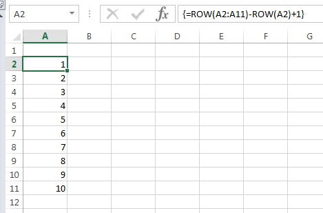
Let’s look at an example, say we want to return a list of numbers 1 through 10 in cells A1:A10.

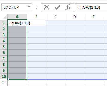
Step 1 – very important; first select cells A1 to A10

Step 2 – type in this formula; =ROW(1:10)

It should look like the image below with the formula in cell A1:

Tip: ROW(A1:A10) or ROW($A$1:$A$10) yields the same results as ROW(1:10).

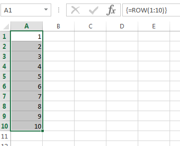
Step 3 – press CTRL+SHIFT+ENTER to complete the formula.

You should have the numbers 1 through 10 in cells A1:A10 and in the formula bar you’ll see the curly braces around your formula as shown below:

Features of Excel Multi-cell Array Formulas

1. If you select any of the cells in the range A1:A10 you’ll see the formula is exactly the same. In effect the range 1:10 is absolute yet I haven’t had to use the $ sign to lock them in.
2. If you try to delete or insert cells or rows between A1:A10 you’ll get this error:
3. To select all of the cells relating to the array formula select one cell containing the formula and press CTRL+/

   

4. To edit the formula simply click on any of the cells in the array, make your changes and press CTRL+SHIFT+ENTER to re-enter the formula.
5. To delete a multi-cell array formula first select the array, in this case cells A1:A10 (remember the keyboard shortcut is CTRL+/), then press DELETE. Alternatively you can delete all of the rows or the column containing the formula.

Multi-cell Array Formula Gotchas

While you can’t insert rows or cells within an array, you can insert rows above and this may alter the results of your formula. For example, if I insert a row above cell A1 my formulas and cell references adjust like so:

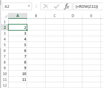
This can be catastrophic for your formula, especially if you’re nesting ROW in another formula and the impact is not transparent like the example above.

The solution is to use this formula instead of ROW(1:10):

=ROW(A1:A10)-ROW(A1)+1

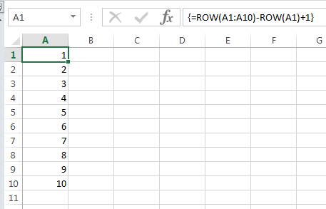
Now when I insert a row above A1 my formula adjusts but I still get numbers 1 through 10:

Tip: you can insert numbers 1 through 10 across a row with this multi-cell array formula:

=COLUMN(A1:J1)-COLUMN(A1)+1

Don’t forget to press CTRL+SHIFT+ENTER to complete the formula.

When to use Multi-cell Array Formulas

We could just as easily insert the numbers 1 through 10 in column A with this formula (entered in any cell):

=ROW(A1)

Then copy down as needed. Of course this formula is subject to error if rows are inserted above it, so you’re better off using the ROWS function like this:

=ROWS($A$1:A1) or =ROWS($1:1)

And don’t forget there’s always Auto-fill or Fill Series for a quick list of numbers.

However, the benefit of using a multi-cell array formula is that it prevents rows/cells being inserted within the range without the need for worksheet protection.

Multi-cell Array Formula Examples

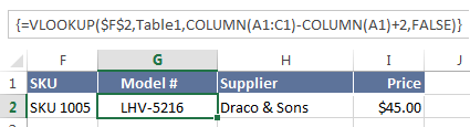
So far we’ve looked at a basic example, but often you’ll find more complex multi-cell array formulas that contain nested functions like this VLOOKUP with COLUMN in cells G2:I2:

I’ll explain; I have an Excel Table in cells A1:D6 called Table1:

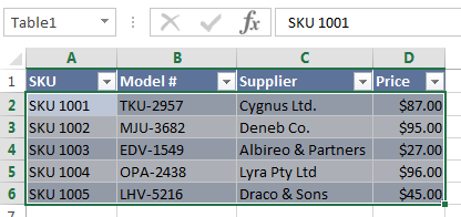
And in cell F2 I have a data validation list containing the SKU’s:

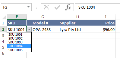
When I choose an SKU from the Data Validation list a multi-cell VLOOKUP array formula in cells G2:I2 returns the Model#, Supplier and Price for the selected SKU:

The only difference between this multi-cell VLOOKUP array formula and a regular VLOOKUP formula is the COLUMN functions used to return the col_index_num argument for VLOOKUP.

When evaluated COLUMN returns an array {2,3,4} for the col_index_num, as you can see below:

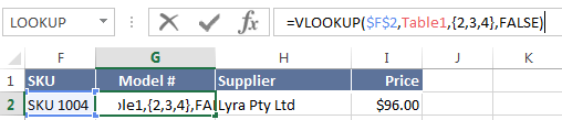
And because I’ve selected 3 cells for my multi-cell array formula it returns the value from 2^nd column in Table1 to cell G2, the value from the 3^rd column in H2 and the value from the 4^th column in I2.

Remember the main benefit of this formula over a regular VLOOKUP is that you can’t insert columns between G and I.

The other benefit is that if an inexperienced user attempts to edit this formula they’re likely to get the error message “you cannot change part of an array”, and that might just be enough to prevent them from messing up your formulas. No promises though. Those users can be tenacious 😉

Multi-cell Array Formula Functions

There are also quite a few functions in Excel that return an array of results. That is they return multiple values and deposit each one in its own cell.

For example the FREQUENCY function does this. The syntax is:

FREQUENCY(data_array, bins_array)

FREQUENCY calculates how often values occur within a range (data_array), for each value in the bins_array. Let’s look at an example:

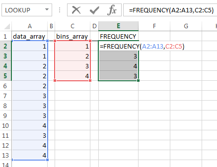
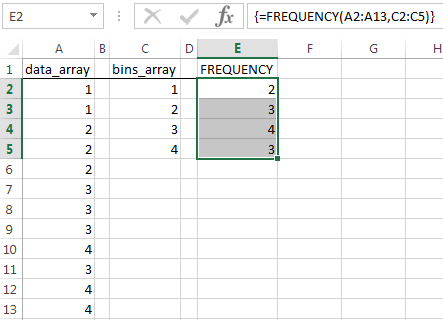
Column A contains a series of values (our data_array). We want to count how often each number in column A occurs. In column C we have our bins_array, which is simply a list of distinct numbers from column A.

In column E we enter our FREQUENCY formula by first selecting 4 cells (E2:E5, one for each bin), then the formula:

=FREQUENCY(A2:A13,C2:C5)

Press CTRL+SHIFT+ENTER to complete the formula.

The image below shows the FREQUENCY formula has counted 2 occurrences of the number 1 in our data_array, 3 occurrences of number 2 and so on:

Advantages of multi-cell array formulas

• User error more easily avoided since editing them is difficult unless you know how.
• Prevents inserting rows/columns within the array range, but not above or below.

Caution

Array formulas applied to large data sets can be slow and inefficient so use them with caution.

Thanks

Thanks to Mike Girvin and his incredible book CTRL+SHIFT+ENTER Mastering Excel Array Formulas. I learnt endless tips in this book. It’s a must read for any Excel enthusiast.

Thanks to Simlaoui’s comment on last week’s post on the ROW function which inspired me to write about multi-cell array formulas.

Disclosure: if you purchase Mike’s book I earn a couple of dollars. That’s not why I recommend it though. It’s a brilliant book and you’ll learn a lot, even if you’re already familiar with array formulas.

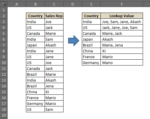
Can we look-up and return multiple values in one cell in Excel (separated by comma or space)?

I have been asked this question multiple times by many of my colleagues and readers.

Excel has some amazing lookup formulas, such as VLOOKUP, INDEX/MATCH (and now XLOOKUP), but none of these offer a way to return multiple matching values. All of these work by identifying the first match and return that.

So I did a bit of VBA coding to come up with a custom function (also called a User Defined Function) in Excel.

Update: After Excel released dynamic arrays and awesome functions such as UNIQUE and TEXTJOIN, it’s now possible to use a simple formula and return all the matching values in one cell (covered in this tutorial).

In this tutorial, I will show you how to do this (if you’re using the latest version of Excel – Microsoft 365 with all the new functions), as well as a way to do this in case you’re using older versions (using VBA).

So let’s get started!

Lookup and Return Multiple Values in One Cell (Using Formula)

If you’re using Excel 2016 or prior versions, go to the next section where I show how to do this using VBA. 

With Microsoft 365 subscription, your Excel now has a lot more powerful functions and features that are not there in prior versions (such as XLOOKUP, Dynamic Arrays, UNIQUE/FILTER functions, etc.)

So if you’re using Microsoft 365 (earlier known as Office 365), you can use the methods covered in this section could look up and return multiple values in one single cell in Excel.

And as you will see, it’s a really simple formula.

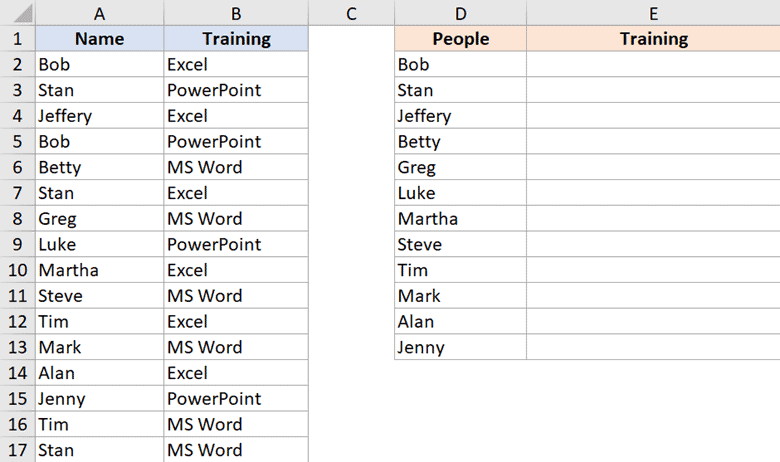
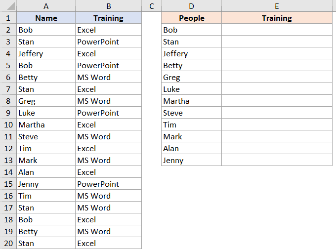
Below I have a data set where I have the names of the people in column A and the training that they have taken in column B.

Click here to download the example file and follow along

For each person, I want to find out what training they have completed. In column D, I have the list of unique names (from column A), and I want to quickly lookup and extract all the training that every person has done and get these in a single set (separated by a comma).

Below is the formula that will do this:

=TEXTJOIN(", ",TRUE,IF(D2=$A$2:$A$20,$B$2:$B$20,""))

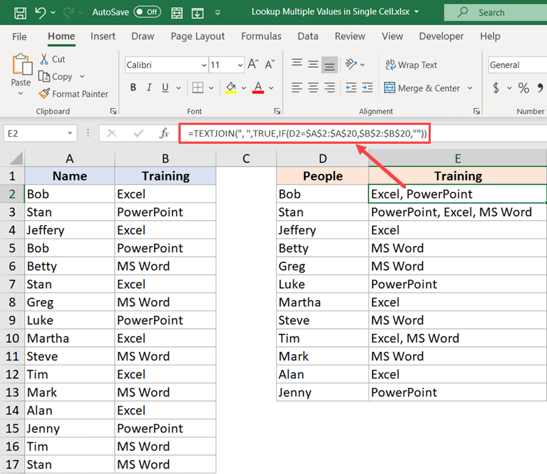
After entering the formula in cell E2, copy it for all the cells where you want the results.

How does this formula work?

Let me deconstruct this formula and explain each part in how it comes together gives us the result.

The logical test in the IF formula (D2=$A$2:$A$20) checks whether the name cell D2 is the same as that in range A2:A20.

It goes through each cell in the range A2:A20, and checks whether the name is the same in cell D2 or not. if it’s the same name, it returns TRUE, else it returns FALSE.

So this part of the formula will give you an array as shown below:

{TRUE;FALSE;FALSE;TRUE;FALSE;FALSE;FALSE;FALSE;FALSE;FALSE;FALSE;FALSE;FALSE;FALSE;FALSE;FALSE;FALSE;FALSE;FALSE}

Since we only want to get the training for Bob (the value in cell D2), we need to get all the corresponding training for the cells that are returning TRUE in the above array.

This is easily done by specifying [value_if_true] part of the IF formula as the range that has the training. This makes sure that if the name in cell D2 matches the name in the range A2:A20, the IF formula would return all the training that person has taken.

And wherever the array returns a FALSE, we have specified the [value_if_false] value as “” (blank), so it returns a blank.

The IF part of the formula returns the array as shown below:

{“Excel”;””;””;”PowerPoint”;””;””;””;””;””;””;””;””;””;””;””;””;””;””;””}

Where it has the names of the training Bob has taken and blanks wherever the name was not Bob.

Now, all we need to do is combine these training name (separated by a comma) and return it in one cell.

And that can easily be done using the new TEXTJOIN formula (available in Excel 2019 and Excel in Microsoft 365)

The TEXTJOIN formula takes three arguments:

• the Delimiter – which is “, ” in our example, as I want the training to separated by a comma and a space character
• TRUE – which tells the TEXTJOIN formula to ignore empty cells and only combine ones that are not empty
• The If formula that returns the text that needs to be combined

If you’re using Excel in Microsoft 365 that already has dynamic arrays, you can just enter the above formula and hit enter. And if you’re using Excel 2019, you need to enter the formula, and hold the Control and the Shift key and then press Enter

Click here to download the example file and follow along

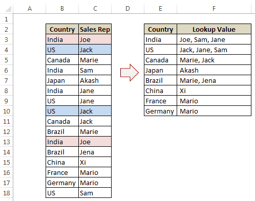
Get Multiple Lookup Values in a Single Cell (without repetition)

Since the UNIQUE formula is only available fro Excel in Microsoft 365, you won’t be able to use this method in Excel 2019

In case there are repetitions in your data set, as shown below, you need to change the formula a little bit so that you only get a list of unique values in a single cell.

In the above data set, some people have taken training multiple times. For example, Bob and Stan have taken the Excel training twice, and  Betty has taken MS Word training twice. But in our result, we do not want to have a training name repeat.

You can use the below formula to do this:

=TEXTJOIN(", ",TRUE,UNIQUE(IF(D2=$A$2:$A$20,$B$2:$B$20,"")))

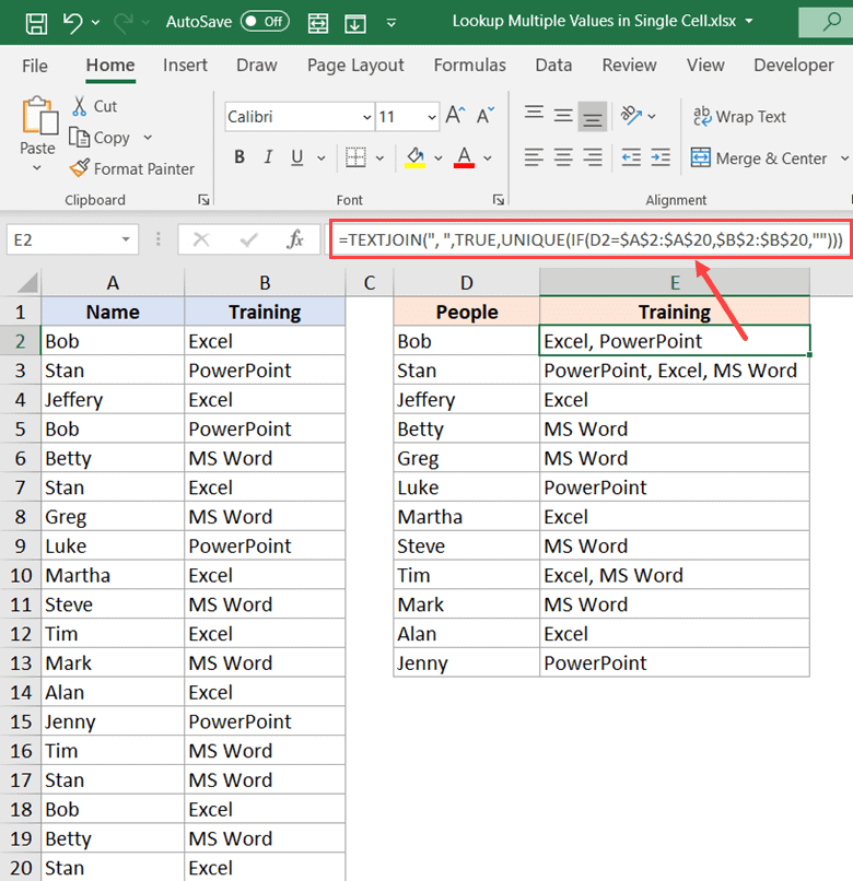
The above formula works the same way, with a minor change. we have used the IF formula within the UNIQUE function so that in case there are repetitions in the if formula result, the UNIQUE function would remove it.

Click here to download the example file

Lookup and Return Multiple Values in One Cell (Using VBA)

If you’re using Excel 2016 or prior versions, then you will not have access to the TEXTJOIN formula. So the best way to then look up and get multiple matching values in a single cell is by using a custom formula that you can create using VBA. 

To get multiple lookup values in a single cell, we need to create a function in VBA (similar to the VLOOKUP function) that checks each cell in a column and if the lookup value is found, adds it to the result.

Here is the VBA code that can do this:

'Code by Sumit Bansal (https://trumpexcel.com)
Function SingleCellExtract(Lookupvalue As String, LookupRange As Range, ColumnNumber As Integer)
  Dim i As Long
  Dim Result As String
  For i = 1 To LookupRange.Columns(1).Cells.Count
  If LookupRange.Cells(i, 1) = Lookupvalue Then
  Result = Result & " " & LookupRange.Cells(i, ColumnNumber) & ","
  End If
  Next i
  SingleCellExtract = Left(Result, Len(Result) – 1)
  End Function

Where to Put this Code?

1. Open a workbook and click Alt + F11 (this opens the VBA Editor window).
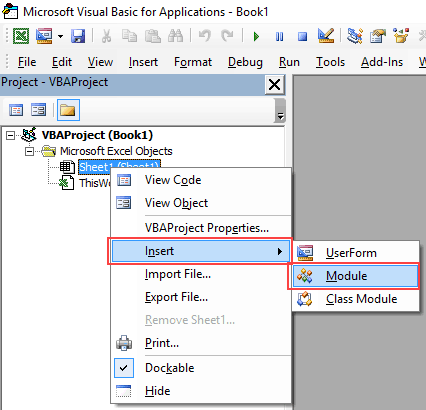
2. In this VBA Editor window, on the left, there is a project explorer (where all the workbooks and worksheets are listed). Right-click on any object in the workbook where you want this code to work, and go to Insert –> Module.
3. In the module window (that will appear on the right), copy and paste the above code.
4. Now you are all set. Go to any cell in the workbook and type =SingleCellExtract and plug in the required input arguments (i.e., LookupValue, LookupRange, ColumnNumber).

How does this formula work?

This function works similarly to the VLOOKUP function.

It takes 3 arguments as inputs:

1. Lookupvalue – A string that we need to look-up in a range of cells.
2. LookupRange  – An array of cells from where we need to fetch the data ($B3:$C18 in this case).
3. ColumnNumber – It is the column number of the table/array from which the matching value is to be returned (2 in this case).

When you use this formula, it checks each cell in the leftmost column in the lookup range and when it finds a match, it adds to the result in the cell in which you have used the formula.

Remember: Save the workbook as a macro-enabled workbook (.xlsm or .xls) to reuse this formula again. Also, this function would be available only in this workbook and not in all workbooks.

Click here to download the example file

Learn how to automate boring repetitive tasks with VBA in Excel. Join the Excel VBA Course

Get Multiple Lookup Values in a Single Cell (without repetition)

There is a possibility that you may have repetitions in the data.

If you use the code used above, it will give you repetitions in the result as well.

If you want to get the result where there are no repetitions, you need to modify the code a bit.

Here is the VBA code that will give you multiple lookup values in a single cell without any repetitions.

'Code by Sumit Bansal (https://trumpexcel.com)
Function MultipleLookupNoRept(Lookupvalue As String, LookupRange As Range, ColumnNumber As Integer)
Dim i As Long
Dim Result As String
For i = 1 To LookupRange.Columns(1).Cells.Count
  If LookupRange.Cells(i, 1) = Lookupvalue Then
    For J = 1 To i - 1
    If LookupRange.Cells(J, 1) = Lookupvalue Then
      If LookupRange.Cells(J, ColumnNumber) = LookupRange.Cells(i, ColumnNumber) Then
        GoTo Skip
      End If
    End If
    Next J
    Result = Result & " " & LookupRange.Cells(i, ColumnNumber) & ","
Skip:
  End If
Next i
MultipleLookupNoRept = Left(Result, Len(Result) - 1)
End Function

Once you have placed this code in the VB Editor (as shown above in the tutorial), you will be able to use the MultipleLookupNoRept function.

Here is a snapshot of the result you will get with this MultipleLookupNoRept function.

Click here to download the example file

In this tutorial, I covered how to use formulas and VBA in Excel to find and return multiple lookup values in one cell in Excel.

While it can easily be done with a simple formula if you’re using Excel in Microsoft 365 subscription, if you’re using prior versions and don’t have access to functions such as TEXTJOIN, you can still do this using VBA by creating your own custom function.

You May Also Like the Following Excel Tutorials:

• How to Create and Use an Excel Add-in.
• How to Run a Macro in Excel.
• Find the Last Occurrence of a Lookup Value a List in Excel
• How to Use VLOOKUP with Multiple Criteria
• How to Record a Macro in Excel – A Step by Step Guide.
• Test Multiple Conditions Using Excel IFS Function

You might want to split a cell into two smaller cells within a single column. Unfortunately, you can’t do this in Excel. Instead, create a new column next to the column that has the cell you want to split and then split the cell. You can also split the contents of a cell into multiple adjacent cells.

See the following screenshots for an example:

Split the content from one cell into two or more cells

1. Select the cell or cells whose contents you want to split.

   Important: When you split the contents, they will overwrite the contents in the next cell to the right, so make sure to have empty space there.

2. On the Data tab, in the Data Tools group, click Text to Columns. The Convert Text to Columns Wizard opens.

   

3. Choose Delimited if it is not already selected, and then click Next.

4. Select the delimiter or delimiters to define the places where you want to split the cell content. The Data preview section shows you what your content would look like. Click Next.

   

5. In the Column data format area, select the data format for the new columns. By default, the columns have the same data format as the original cell. Click Finish.

See Also

Merge and unmerge cells

Merging and splitting cells or data

See all How-To Articles

This tutorial demonstrates how to add values to cells and columns in Excel and Google Sheets.

Add Values to Multiple Cells

1. To add a value to a range of cells, click on the cell where you want to display the result, and enter = (equal) and the cell reference of the first number then + (plus) and the number you want to add.

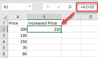
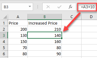
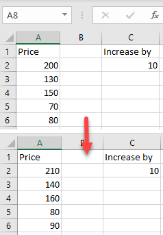
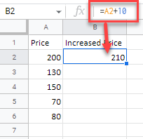
For this example, start with cell A2 (200). Cell B2 will show the Price in A2 increased by 10. So, in cell B2, enter:

=A2+10

As a result, the value in cell B2 is now 210 (value from A2 plus 10).

1. Now copy this formula down the column to the rows below. Click on the cell where you entered the formula (F2) and place your cursor on the bottom right corner of the cell.
2. When it changes to a plus sign, drag it down to the rest of the rows where you want to apply the formula (here, B2:B6).

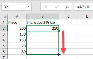
As a result of relative cell referencing, the constant (here, 10) remains the same, but the cell address changes according to the row you are in (so B3=A3+10, and so on).

Add Multiple Cells With Paste Special

You can also add a number to multiple cells and return the result as a number in the same cell.

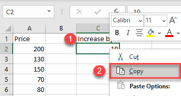
1. First, select the cell with the value you want to add (here, cell C2), right-click, and from the drop-down menu, choose Copy (or use the shortcut CTRL + C).

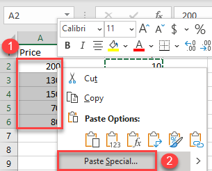
1. After that, select the cells where you want to subtract the value and right-click on the data range (here, A2:A6). In the drop-down menu, click on Paste Special.

1. The Paste Special window will appear. Under the Operation section choose Add, and then click OK.

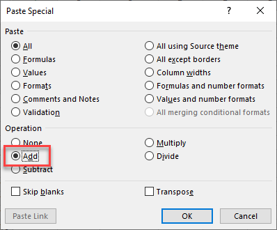
You’ll see the result as a number within the same cells. (In this example, 10 was added to each value from the data range A2:A6.) This method is better if you don’t want to display the results in a new column and don’t need to retain a record of the original values.

Add Column With Cell References

To add an entire column to another using cell references, select the cell where you want to display the result, and enter = (equal) and the cell reference for the first number then + (plus) and the reference for the cell you want to add.

For this example, calculate the summary of Price 1 (A2) and Price 2 (B2). So, in cell C2, enter:

=A2+B2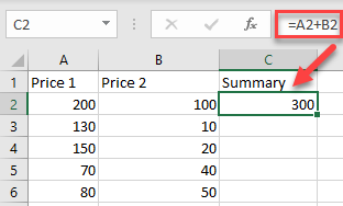

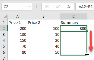
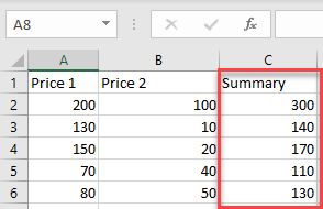
To apply the formula to an entire column, just copy the formula down to the rest of the rows in the table (here, C2:C6).

Now, you have a new column with the summary.

Using the methods above, you can also subtract, multiply, or divide cells and columns in Excel.

Add Cells and Columns in Google Sheets

In Google Sheets, you can add multiple cells using formulas in exactly the same ways as in Excel; except, you can’t use Paste Special.

Combining values with CONCATENATE is the best way, but with this function, it’s not possible to refer to an entire range.

You need to select all the cells of a range one by one, and if you try to refer to an entire range, it will return the text from the first cell.

In this situation, you do need a method where you can refer to an entire range of cells to combine them in a single cell.

So today in this post, I’d like to share with you 5 different ways to combine text from a range into a single cell.

[CONCATENATE + TRANSPOSE] to Combine Values

The best way to combine text from different cells into one cell is by using the transpose function with concatenating function.

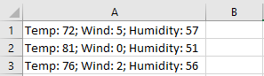
Look at the below range of cells where you have a text but every word is in a different cell and you want to get it all in one cell.

Below are the steps you need to follow to combine values from this range of cells into one cell.

1. In the B8 (edit the cell using F2), insert the following formula, and do not press enter.
   • =CONCATENATE(TRANSPOSE(A1:A5)&” “)
2. Now, select the entire inside portion of the concatenate function and press F9. It will convert it into an array.
3. After that, remove the curly brackets from the start and the end of the array.
4. In the end, hit enter.

That’s all.

How this formula works

In this formula, you have used TRANSPOSE and space in the CONCATENATE. When you convert that reference into hard values it returns an array.

In this array, you have the text from each cell and a space between them and when you hit enter, it combines all of them.

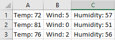
Combine Text using the Fill Justify Option

Fill justify is one of the unused but most powerful tools in Excel. And, whenever you need to combine text from different cells you can use it.

The best thing is, that you need a single click to merge text. Have look at the below data and follow the steps.

1. First of all, make sure to increase the width of the column where you have text.
2. After that, select all the cells.
3. In the end, go to Home Tab ➜ Editing ➜ Fill ➜ Justify.

This will merge text from all the cells into the first cell of the selection.

TEXTJOIN Function for CONCATENATE Values

If you are using Excel 2016 (Office 365), there is a function called “TextJoin”. It can make it easy for you to combine text from different cells into a single cell.

Syntax:

TEXTJOIN(delimiter, ignore_empty, text1, [text2], …)

1. delimiter a text string to use as a delimiter.
2. ignore_empty true to ignore blank cell, false to not.
3. text1 text to combine.
4. [text2] text to combine optional.

how to use it

To combine the below list of values you can use the formula:

=TEXTJOIN(" ",TRUE,A1:A5)

Here you have used space as a delimiter, TRUE to ignore blank cells and the entire range in a single argument. In the end, hit enter and you’ll get all the text in a single cell.

Combine Text with Power Query

Power Query is a fantastic tool and I love it. Make sure to check out this (Excel Power Query Tutorial). You can also use it to combine text from a list in a single cell. Below are the steps.

1. Select the range of cells and click on “From table” in data tab.
   
2. If will edit your data into Power Query editor.
   
3. Now from here, select the column and go to “Transform Tab”.
4. From “Transform” tab, go to Table and click on “Transpose”.
   
5. For this, select all the columns (select first column, press and hold shift key, click on the last column) and press right click and then select “Merge”.
   
6. After that, from Merge window, select space as a separator and name the column.
   
7. In the end, click OK and click on “Close and Load”.

Now you have a new worksheet in your workbook with all the text in a single cell. The best thing about using Power Query is you don’t need to do this setup again and again.

When you update the old list with a new value you need to refresh your query and it will add that new value to the cell.

VBA Code to Combine Values

If you want to use a macro code to combine text from different cells then I have something for you. With this code, you can combine text in no time. All you need to do is, select the range of cells where you have the text and run this code.

 Sub combineText()
 Dim rng As Range
 Dim i As String
 For Each rng In Selection
 i = i & rng & " "
 Next rng
 Range("B1").Value = Trim(i)
 End Sub 

Make sure to specify your desired location in the code where you want to combine the text.

In the end,

There may be different situations for you where you need to concatenate a range of cells into a single cell. And that’s why we have these different methods.

All methods are easy and quick, you need to select the right method as per your need. I must say that give a try to all the methods once and tell me:

Which one is your favorite and worked for you?

Please share your views with me in the comment section. I’d love to hear from you, and please, don’t forget to share this post with your friends, I am sure they will appreciate it.