
Excel 2021 Excel 2019 Excel 2016 Excel 2013 Office for business Excel 2010 More…Less
Summary
When you use the Microsoft Excel products listed at the bottom of this article, you can use a worksheet formula to covert data that spans multiple rows and columns to a database format (columnar).
More Information
The following example converts every four rows of data in a column to four columns of data in a single row (similar to a database field and record layout). This is a similar scenario as that which you experience when you open a worksheet or text file that contains data in a mailing label format.
Example
-
In a new worksheet, type the following data:
A1: Smith, John
A2: 111 Pine St.
A3: San Diego, CA
A4: (555) 128-549
A5: Jones, Sue
A6: 222 Oak Ln.
A7: New York, NY
A8: (555) 238-1845
A9: Anderson, Tom
A10: 333 Cherry Ave.
A11: Chicago, IL
A12: (555) 581-4914 -
Type the following formula in cell C1:
=OFFSET($A$1,(ROW()-1)*4+INT((COLUMN()-3)),MOD(COLUMN()-3,1))
-
Fill this formula across to column F, and then down to row 3.
-
Adjust the column sizes as necessary. Note that the data is now displayed in cells C1 through F3 as follows:
Smith, John
111 Pine St.
San Diego, CA
(555) 128-549
Jones, Sue
222 Oak Ln.
New York, NY
(555) 238-1845
Anderson, Tom
333 Cherry Ave.
Chicago, IL
(555) 581-4914
The formula can be interpreted as
OFFSET($A$1,(ROW()-f_row)*rows_in_set+INT((COLUMN()-f_col)/col_in_set), MOD(COLUMN()-f_col,col_in_set))
where:
-
f_row = row number of this offset formula
-
f_col = column number of this offset formula
-
rows_in_set = number of rows that make one record of data
-
col_in_set = number of columns of data
Need more help?
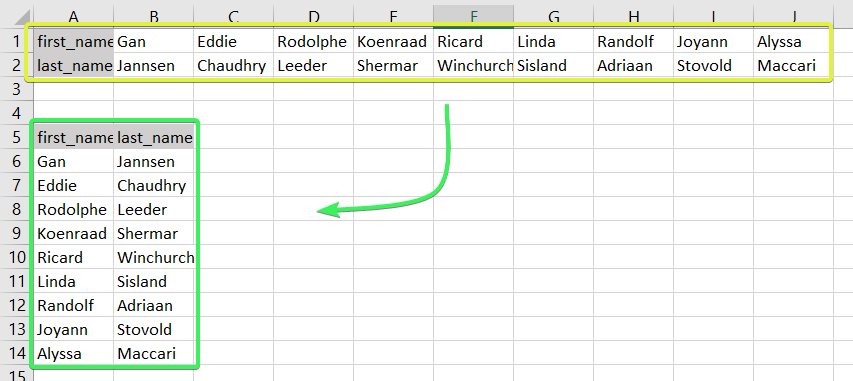
Do you have some values arranged as rows in your workbook, and do you want to convert text in rows to columns in Excel like this?
In Excel, you can do this manually or automatically in multiple ways depending on your purpose. Read on to get all the details and choose the best solution for yourself.
How to convert rows into columns or columns to rows in Excel – the basic solution
The easiest way to convert rows to columns in Excel is via the Paste Transpose option. Here is how it looks:
- Select and copy the needed range
- Right-click on a cell where you want to convert rows to columns
- Select the Paste Transpose option to rotate rows to columns
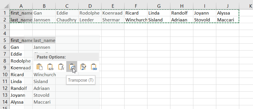
As an alternative, you can use the Paste Special option and mark Transpose using its menu.

It works the same if you need to convert columns to rows in Excel.

This is the best way for a one-time conversion of small to medium numbers of rows both in the Excel desktop and online.
Can I convert multiple rows to columns in Excel from another workbook?
The method above will work well if you want to convert rows to columns in Excel between different workbooks using Excel desktop. You need to have both spreadsheets open and do the copying and pasting as described.
However, in Excel Online, this won’t work for different workbooks. The Paste Transpose option is not available.
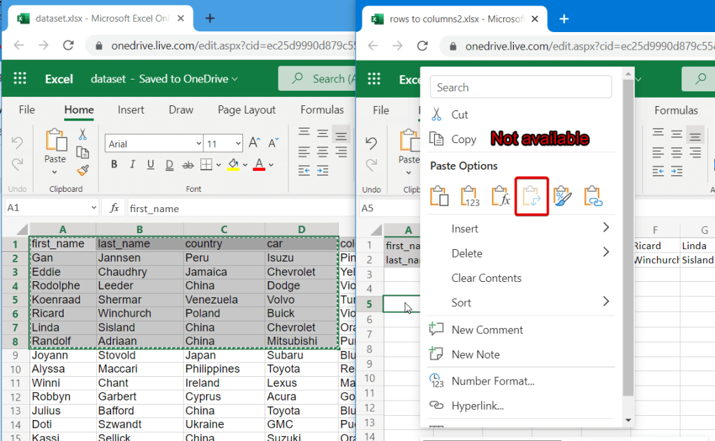
Therefore, in this case, it’s better to use the TRANSPOSE function.
How to switch rows and columns in Excel in more efficient ways
To switch rows and columns in Excel automatically or dynamically, you can use one of these options:
- Excel TRANSPOSE function
- VBA macro
- Power Query
Let’s check out each of them in the example of a data range that we imported to Excel from a Google Sheets file using Coupler.io.

Coupler.io is an integration solution that synchronizes data between source and destination apps on a regular schedule. For example, you can set up an automatic data export from Google Sheets every day to your Excel workbook.
Check out all the available Excel integrations.

How to change row to column in Excel with TRANSPOSE
TRANSPOSE is the Excel function that allows you to switch rows and columns in Excel. Here is its syntax:
=TRANSPOSE(array)array– an array of columns or rows to transpose
One of the main benefits of TRANSPOSE is that it links the converted columns/rows with the source rows/columns. So, if the values in the rows change, the same changes will be made in the converted columns.
TRANSPOSE formula to convert multiple rows to columns in Excel desktop
TRANSPOSE is an array formula, which means that you’ll need to select a number of cells in the columns that correspond to the number of cells in the rows to be converted and press Ctrl+Shift+Enter.
=TRANSPOSE(A1:J2)
Fortunately, you don’t have to go through this procedure in Excel Online.
TRANSPOSE formula to rotate row to column in Excel Online
You can simply insert your TRANSPOSE formula in a cell and hit enter. The rows will be rotated to columns right away without any additional button combinations.
Excel TRANSPOSE multiple rows in a group to columns between different workbooks
We promised to demonstrate how you can use TRANSPOSE to rotate rows to columns between different workbooks. In Excel Online, you need to do the following:
- Copy a range of columns to rotate from one spreadsheet and paste it as a link to another spreadsheet.

- We need this URL path to use in the TRANSPOSE formula, so copy it.

- The URL path above is for a cell, not for an array. So, you’ll need to slightly update it to an array to use in your TRANSPOSE formula. Here is what it should look like:
=TRANSPOSE('https://d.docs.live.net/ec25d9990d879c55/Docs/Convert rows to columns/[dataset.xlsx]dataset'!A1:D12)

You can follow the same logic for rotating rows to columns between workbooks in Excel desktop.
Are there other formulas to convert columns to rows in Excel?
TRANSPOSE is not the only function you can use to change rows to columns in Excel. A combination of INDIRECT and ADDRESS functions can be considered as an alternative, but the flow to convert rows to columns in Excel using this formula is much trickier. Let’s check it out in the following example.
How to convert text in columns to rows in Excel using INDIRECT+ADDRESS
If you have a set of columns with the first cell A1, the following formula will allow you to convert columns to rows in Excel.
=INDIRECT(ADDRESS(COLUMN(A1),ROW(A1)))

But where are the rows, you may ask! Well, first you need to drag this formula down if you are converting multiple columns to rows. Then drag it to the right.

NOTE: This Excel formula only to convert data in columns to rows starting with A1 cell. If your columns start from another cell, check out the next section.
How to convert Excel data in columns to rows using INDIRECT+ADDRESS from other cells
To convert columns to rows in Excel with INDIRECT+ADDRESS formulas from not A1 cell only, use the following formula:
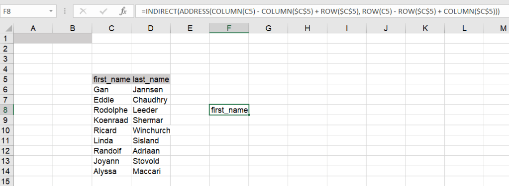
=INDIRECT(ADDRESS(COLUMN(first_cell) - COLUMN($first_cell) + ROW($first_cell), ROW(first_cell) - ROW($first_cell) + COLUMN($first_cell)))
- first_cell – enter the first cell of your columns
Here is an example of how to convert Excel data in columns to rows:
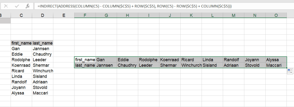
=INDIRECT(ADDRESS(COLUMN(C5) - COLUMN($C$5) + ROW($C$5), ROW(C5) - ROW($C$5) + COLUMN($C$5)))
Again, you’ll need to drag the formula down and to the right to populate the rest of the cells.
How to automatically convert rows to columns in Excel VBA
VBA is a superb option if you want to customize some function or functionality. However, this option is only code-based. Below we provide a script that allows you to change rows to columns in Excel automatically.
- Go to the Visual Basic Editor (VBE). Click Alt+F11 or you can go to the Developer tab => Visual Basic.

- In VBE, go to Insert => Module.
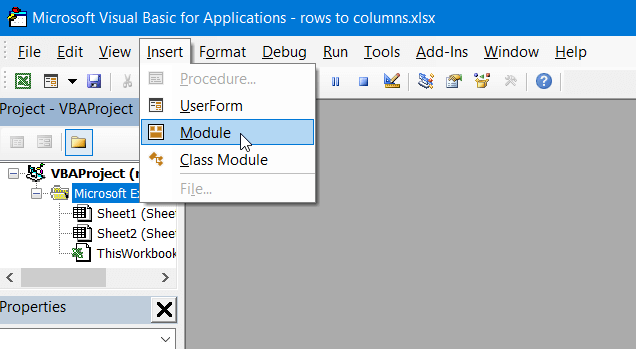
- Copy and paste the script into the window. You’ll find the script in the next section.

- Now you can close the VBE. Go to Developer => Macros and you’ll see your RowsToColumns macro. Click Run.

- You’ll be asked to select the array to rotate and the cell to insert the rotated columns.

- There you go!

VBA macro script to convert multiple rows to columns in Excel
Sub TransposeColumnsRows()
    Dim SourceRange As Range
    Dim DestRange As Range

    Set SourceRange = Application.InputBox(Prompt:="Please select the range to transpose", Title:="Transpose Rows to Columns", Type:=8)
    Set DestRange = Application.InputBox(Prompt:="Select the upper left cell of the destination range", Title:="Transpose Rows to Columns", Type:=8)

    SourceRange.Copy
    DestRange.Select
    Selection.PasteSpecial Paste:=xlPasteAll, Operation:=xlNone, SkipBlanks:=False, Transpose:=True
    Application.CutCopyMode = False

End Sub

Sub RowsToColumns()
    Dim SourceRange As Range
    Dim DestRange As Range

    Set SourceRange = Application.InputBox(Prompt:="Select the array to rotate", Title:="Convert Rows to Columns", Type:=8)
    Set DestRange = Application.InputBox(Prompt:="Select the cell to insert the rotated columns", Title:="Convert Rows to Columns", Type:=8)

    SourceRange.Copy
    DestRange.Select
    Selection.PasteSpecial Paste:=xlPasteAll, Operation:=xlNone, SkipBlanks:=False, Transpose:=True
    Application.CutCopyMode = False

End Sub
Read more in our Excel Macros Tutorial.
Convert rows to column in Excel using Power Query
Power Query is another powerful tool available for Excel users. We wrote a separate Power Query Tutorial, so feel free to check it out.
Meanwhile, you can use Power Query to transpose rows to columns. To do this, go to the Data tab, and create a query from table.

- Then select a range of cells to convert rows to columns in Excel. Click OK to open the Power Query Editor.

- In the Power Query Editor, go to the Transform tab and click Transpose. The rows will be rotated to columns.
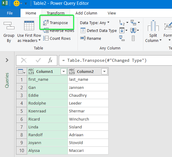
- If you want to keep the headers for your columns, click the Use First Row as Headers button.
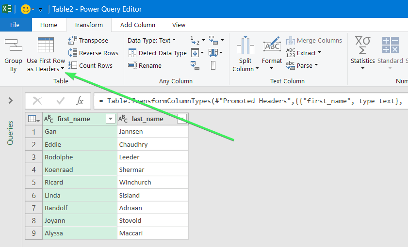
- That’s it. You can Close & Load your dataset – the rows will be converted to columns.

Error message when trying to convert rows to columns in Excel
To wrap up with converting Excel data in columns to rows, let’s review the typical error messages you can face during the flow.
Overlap error

The overlap error occurs when you’re trying to paste the transposed range into the area of the copied range. Please avoid doing this.
Wrong data type error

You may see this #VALUE! error when you implement the TRANSPOSE formula in Excel desktop without pressing Ctrl+Shift+Enter.
Other errors may be caused by typos or other misprints in the formulas you use to convert groups of data from rows to columns in Excel. Always double-check the syntax before pressing Enter or Ctrl+Shift+Enter 🙂 . Good luck with your data!
-

A content manager at Coupler.io whose key responsibility is to ensure that the readers love our content on the blog. With 5 years of experience as a wordsmith in SaaS, I know how to make texts resonate with readers’ queries✍🏼

Back to Blog
Focus on your business
goals while we take care of your data!
Try Coupler.io
Excel Rows to Columns (Table of Contents)
- Rows to Columns in Excel
- How to Convert Rows to Columns in Excel using Transpose?
Rows to Columns in Excel
In Microsoft Excel, we can change the rows to column and column to row vice versa, using TRANSPOSE. We can either use the Transpose or Transpose function to get the output.
Definition of Transpose
Transpose function normally returns a transposed range of cells which is used to switch the rows to columns and columns to rows vice versa, i.e. we can convert a vertical range of cells to a horizontal range of cells or a horizontal range of cells to a vertical range of cells in excel.
For example, a horizontal range of cells is returned if a vertical range is entered, or a vertical range of cells is returned if a horizontal range of cells is entered.
How to Convert Rows to Columns in Excel using Transpose?
It is very simple and easy. Let’s understand the working of converting rows to columns in excel by using some examples.
You can download this Convert Rows to Columns Excel?Template here – Convert Rows to Columns Excel?Template
Steps to use transpose:
- Start the cell by selecting and copying an entire range of data.
- Click on the new location.
- Right-click the cell.
- Choose to paste special, and we will find the transpose button.
- Click on the 4th option.
- We will get the result converted to rows to columns.
Example #1
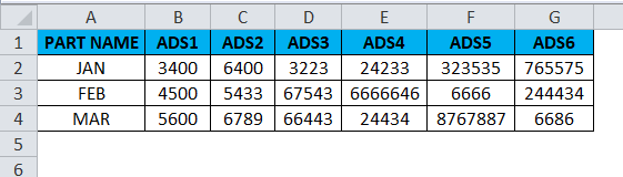
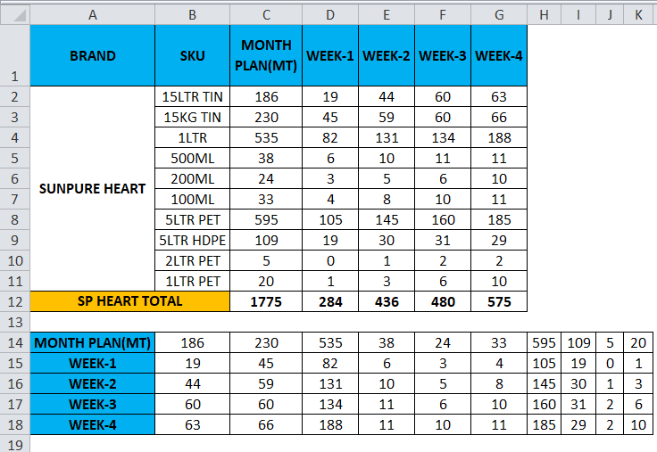
Consider the below example where we have a revenue figure for sales month wise. We can see that month data are row-wise and Part number data are column-wise.
If we want to convert the rows to the column in excel, we can use the transpose function and apply it by following the below steps.
- First, select the entire cells from A To G, which has data information.
- Copy the entire data by pressing the Ctrl+ C Key.
- Now select the new cells where exactly you need to have the data.
- Right, click on the new cell, and we will get the below option which is shown below.

- Choose the option paste special.
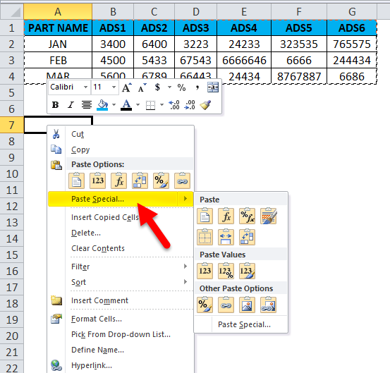
- Select the fourth option in paste special, which is called transpose, as shown in the below screenshot highlighted in yellow color.
- Once we click on transpose, we will get the below output as follows.
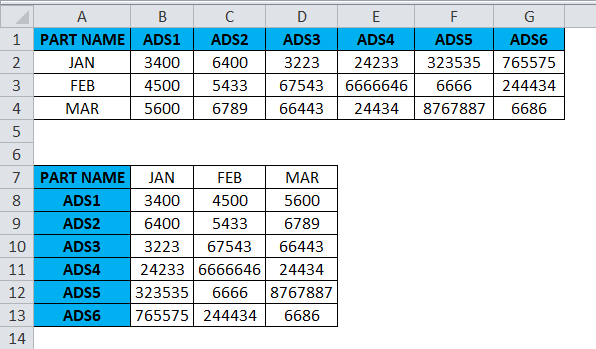
In the above screenshot, we can see that rows have been changed to column and column has been changed to rows in excel. In this way, we can easily convert the given data from row to column and column to row in excel. For the end-user, if there is a huge data, this transpose will be very useful, and it saves a lot of time instead of typing it, and we can avoid duplication.
Example #2
In this example, we will convert rows to the column in excel and see how to use transpose the employee salary data by following the below steps.
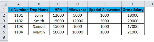
Consider the above screenshot, which has id number, emp name, HRA, Allowance, and Special Allowance. Suppose we need to convert the data column to rows; in these cases TRANSPOSE function will be very useful to convert it, which saves time instead of entering the data. We will see how to convert the column to row with the below steps.
- Click on the cell and copy the entire range of data as shown below.
- Once you copy the data, choose the new cell location.
- Right-click on the cell.
- We will get the paste special dialogue box.
- Choose Paste Special option.
- Select the Transpose option in that, as shown below.
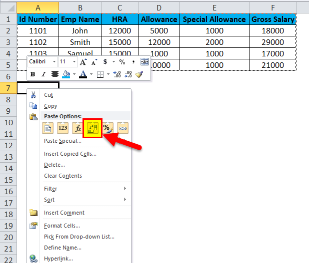
- Once you have chosen the transpose option, the excel row data will be converted to the column as shown in the below result.
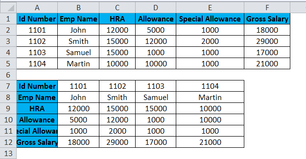
In the above screenshot, we can see the difference that row has been converted to columns; in this way, we can easily use the transpose to convert horizontal to vertical and vertical to horizontal in excel.
Transpose Function
In excel, a built-in function called Transpose Function converts rows to columns and vice versa; this function works the same as transpose. i.e. we can convert rows to columns or columns into rows vice versa.
Syntax of Transpose Function:

Argument
- Array: The range of cells to transpose.
When a set of an array is transposed, the first row is used as the first column of an array, and in the same way, the second row is used as the second column of a new one and the third row is used as the third column of the array.
If we are using the transpose function formula as an array, then we have CTRL+SHIFT +ENTER to apply it.
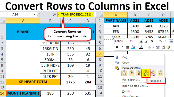
Example #3
In this example, we are going to see how to use the transpose function with an array with the below example.
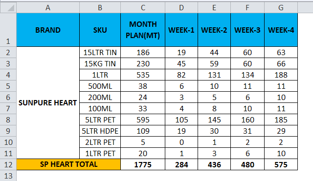
Consider the below example, which shows sales data week wise where we are going to convert the data to columns to row and row to column vice versa by using the transpose function.
- Click on the new cell.
- Select the row you want to transpose.
- Here we are going to convert the MONTH PLAN to the column.
- We can see that there are 11 rows, so in order to use the transpose function, the rows and columns should be in equal cells; if we have 11 rows, then the transpose function needs the same 11 columns to convert it.
- Choose exactly 11 columns, use the Transpose Formula, and select an array from C1 to C11, as shown in the below screenshot.
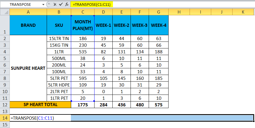
- Now use CTRL+SHIFT +ENTER to apply as an array formula.
- Once we use the CTRL+SHIFT +ENTER, we can see the open and close parenthesis in the formulation.
- We will get the output where a row has been changed to the column, which is shown below.
- Use the formula for the entire cells so that we will get the exact result.
So the Final Output will be as below.
Things to Remember about Convert Rows to Columns in Excel
- Transpose function is one of the most useful functions in excel where we can rotate the data, and the data information will not be changed while converting.
- If there are any blank or empty cells, transpose will not work, and it will give the result as zero.
- While using the array formula in transpose function, we cannot delete or edit the cells because all the data are connected with links, and Excel will throw an error message that “YOU CAN NOT CHANGE PART OF AN ARRAY.”
Recommended Articles
This has been a guide to Rows to Columns in Excel. Here we discuss how to convert rows to columns in excel using transpose along with practical examples and a downloadable excel template. Transpose can help everyone to convert multiple rows to a column in excel easily quickly. You can also go through our other suggested articles –
- Excel COLUMNS Function
- Excel ROW Function
- Unhide Columns in Excel
- Excel Rows and Columns
Defining the Mission
Let’s begin by examining the data then discuss the result we are hoping to achieve.
We have a dataset with three columns: Project, Department, and Person.

The data is in a proper Excel Table format where we have given the table the name “TProject”.
Our objective is to create a two-way table (officially known as a cross-tabular structure); one that lists the Projects to the left and the Departments across the top.

At the intersection of each “Project/Department” combination we wish to see all Persons assigned to the said combination.
Here’s the catch. A typical two-way table would list a separate “Project/Department” entry for each associated Person.

Our table should have but a single entry for each “Project/Department” and list all Persons in a single cell.

We will examine 3 methods for achieving this result, each using a different toolset:
- Formulas
- Power Query
- DAX
I’ll leave it up to you to decide which method works best for you.
Method #1 – Using Formulas
As the two-way table has 3 main components (Project, Department, and Person), we will construct the result in 3 steps.
Step 1: Unique Projects using UNIQUE
We begin by making a list of unique projects. This is accomplished using Excel’s UNIQUE function.
The UNIQUE function will reduce the list of Projects into a single unique list.
Select cell E3 and enter the following formula:
=UNIQUE(TProject[Project])
BONUS FORMULA: If you want your result sorted in alphabetical order, place the previous formula inside a SORT function.
=SORT(UNIQUE(TProject[Project]))
Step 2: Unique Departments using UNIQUE and TRANSPOSE
Next, We make a list of unique departments using Excel’s UNIQUE function.
Because we want the results to be listed “left to right”, we will place the UNIQUE function inside a TRANSPOSE function to perform the “flip”.
Select cell F2 and enter the following formula:
=TRANSPOSE(UNIQUE(TProject[Department]))
As before, you can also integrate the SORT function into this formula to produce an alphabetically sorted list of departments.
=TRANSPOSE(SORT(UNIQUE(TProject[Department])))
Step 3: List Associated Persons for each “Project/Department” Combination
This step is trickier than it appears because some “Project/Department” combinations have more than one Person associated with them.
How can we return every associated Person in a single cell for a given “Project/Department” combination?
Start by thinking of a function that can return multiple results for given criteria.
The FILTER function works well for this need.
In cell F3, write the following FILTER function:
=FILTER(TProject[Person], TProject[Project] & TProject[Department] = E3 & F2, “”)Because we wish to fill this formula down and to the right to create an array of results, we need to “fix” or “lock” the references so that one part of the reference can be modified when copied while the other part remains unchanged.
The modified formula with mixed reference appears as follows.
=FILTER(TProject[Person], TProject[Project] & TProject[Department] = $E3 & F$2, “”)
Note: The two sets of double quotes at the end tell FILTER to show nothing if there are no results for a given “Project/Department” combination.
Dealing with Multiple Results
If we examine the results for “Grand Slam” and “Sales” (cell F3), we see that 2 names are returned.

Because the new Dynamic Array functions will “spill” results into adjacent cells, we need to come up with a way to combine all results into a single cell.
This is where the TEXTJOIN function comes to the rescue.
The TEXTJOIN function will take a list of items and chain them together with a delimiter (i.e., defined characters between each list item.) In our case, we want an ampersand symbol (&) with a leading and trailing space.
“ & ”
The update formula will be of the following structure:
=TEXTJOIN(“ & ”, TRUE, {previous FILTER function goes here} )NOTE: The TRUE tells TEXTJOIN to ignore empty cells. You could leave this out as it is the default behavior, but we’ll include it here just for completeness.
Update the previous formula to include the TEXTJOIN function
=TEXTJOIN(“ & ”, TRUE, FILTER(TProject[Person], TProject[Project] & TProject[Department] = $E3 & F$2, “”) )
Repeating the Formula for the Remainder of the Table
Now that we have our formula working, let’s fill/repeat the formula down and across to the adjacent cells.
If we grab the Fill Series handle and fill down to cell F6, all seems right with the World.

But look what happens when we fill to the right for the remaining Departments.
We don’t see any results. This is because the references to the table columns are moving due to natural Relative Reference behavior.
When referencing columns in an Excel Table, the column name references will change (i.e., “move”) to the next column when using the Fill Series feature.
There is a formulaic way to deal with this, but it is a bit complicated and will cause our formula to increase in size. A simple fix for this is to manually copy/paste the formulas in cells F3:F6 into cells G3:G6 and cells H3:H6.

If you’re feeling adventurous, the below formula is how you would solve this problem in a way that would allow the Fill Series feature to operate as expected.
Don’t say I didn’t warn you.
=TEXTJOIN(" & ", TRUE, FILTER(TProject[[Person]:[Person]], TProject[[Project]:[Project]] & TProject[[Department]:[Department]] = $E3 & F$2, "") )Method #2 – Using Power Query
Power Query is (it could be argued) the best feature in Excel you could devote time to learning.
Transforming “dirty” data into “clean” data is Power Query’s specialty.
Let’s see how Power Query can convert the data into the desired two-way table format.
Bringing the Data into Power Query
To bring the table of data into Power Query, click anywhere in the data and select Data (tab) -> Get & Transform Data (group) -> From Sheet (formerly labeled as “From Table/Range”).

You are presented with the Power Query Editor and a view of the imported data.

Pivoting the Department Column
Because we want the list of Departments across the top of the table, we can select the heading for Department and then click Transform (tab) -> Any Column (group) -> Pivot Column.

In the Pivot Column dialog box, we select Person as the “Values Column” (the column to be aggregated at each “Project/Department” intersection). Also, expand the “Advanced Options” and set the aggregation method to “Don’t Aggregate” and click OK.

The result is less than optimal. Clicking to the right of one of the ERROR entries, we can see in the Preview Window (bottom of the editor) that Power Query can’t display multiple results in a single cell.

We need to come up with a way to join all the related Person entries before performing the pivot column operation.
Since Power Query doesn’t have an Undo feature, we can remove the “Pivot Column” step by clicking the “X” to the left of the step listed in the Applied Steps panel.

Grouping the Persons by Project & Department
Grouping is a great way to create lists of items that share a common factor. In our case, we want to create a separate list of Person names for each “Project/Department” combination.
To do this, select the Project and Department headers (click on “Project”, then hold down CTRL and click on “Department”).
Next, select Home (tab) -> Transform (group) -> Group By.

Because we had pre-selected the “Project” and “Department” columns, these columns are pre-configured as columns to group by.
Change the name of the output column to “Results” and set the Operation to “All Rows”.

We are presented with a table of unique “Project/Department” combinations.

BONUS: Sorting the Projects and Departments
Before we pivot the Department column and create a two-way table, let’s get the list of projects and the list of departments sorted in alphabetical order.
Click the small down-arrow button on the Project column heading and select “Sort Ascending”.

Perform the same step on the Department column.
If you look closely, you can see small up arrows on the buttons and small numbers beside the buttons.

The arrows indicate sort direction (ascending) and the numbers indicate sort order.
All projects are listed in alphabetical order, and if duplicates projects exist, then each duplicated project will be sorted by department.
Creating the Combined Results
We’re still not ready to pivot the Departments because our Results column contains nested tables.
Clicking to the right of any of the nested “Table” entries reveals the complete table rows for the selected “Project/Department” combination.

Our goal is to combine all entries in the Person column of each nested table and display them in a single cell.
To do this, we will create a custom column and use a Power Query function to extract the names for each nested table.
Click Add Column (tab) -> General (group) -> Custom Column.

In the Custom Column dialog box, name the new column “Lists” and enter the following formula in the formula field:
=[Results][Person]
When we click OK, we see a new column with nested lists. Clicking to the right of a List reveals in the Preview Windows the extracted names for that “Project/Department” combination.

Now comes the part where we join the names together, separated by “ & “ characters as we did in the formulas example.
Click the small “left/right” arrow button at the top of the “Lists” column and select “Extract Values…”

In the “Extract values from list” dialog box, select –Custom– and enter the “space ampersand space” character combination. Click OK when finished.

The result is exactly what we are looking for.

Delete the “Results” column by clicking the column heading and press the Delete key on the keyboard.

Pivoting the Departments
Our final step in the creation of this two-way table is to select the Department column heading and execute the Pivot Column operation as we did earlier.
In the Pivot Column dialog box, select “Lists” as the Values Column (the column to be aggregated at each “Project/Department” intersection) and set the aggregation method to “Don’t Aggregate”.

Clicking OK reveals our perfectly formed, two-way table.

Sending the Results to Excel as a Table
To send the results back to Excel as a new table, click Home (tab) -> Close (group) -> Close & Load.

NOTE: If you add/remove/modify entries in the source data, you will need to right-click on the Power Query results and select “Refresh”.
Method #3 – Using DAX Formulas & Power Pivot
Power Pivot is a data modeling technology that lets you create data models, establish relationships, and create calculations.”
Data Analysis Expressions (DAX) is a library of functions and operators that can be combined to build formulas and expressions in Power BI, Analysis Services, and Power Pivot in Excel data models.
We will use Power Pivot and the associated DAX functions to create the two-way table.
Loading the Data into DAX
We begin by loading the data into the Power Pivot Data Model. This is done by clicking anywhere in the data and selecting Power Pivot (tab) -> Tables (group) -> Add to Data Model.

This opens the Power Pivot for Excel window where we can perform a variety of data mode activities.

Before we dive in and start creating measures in our model, let’s step back to “regular” Excel and create a Pivot Table.
From there, we will determine which measures need to be created. We will return to Power Pivot and create the magic.
Close the Power Pivot for Excel window and return to Excel.
Build a Pivot Table
Normally we would click in the data to create a Pivot Table, but since we have loaded the table into the Data Model we will click in the Pivot Table destination call and select Insert (tab) -> Tables (group) -> Pivot Table -> From Data Model.

Select the desired location for the and click OK. We are presented with an empty shell of a Pivot Table.

In the PivotTable Fields panel, place Project in the Rows section and Department in the Columns section.

We can’t place Person in the Values field as it will count the number of entries for each “Project/Department” combination.

Like the previous methods, we want to iterate through the table, concatenating each person with an identical “Project/Department” combination.
DAX has a function that can perform this type of activity; its name is CONCATENATEX.
Creating the Measure using CONCATENATEX
To create a measure in the Data Model that uses CONCATENATEX, right-click on the table name “TProject” in the PivotTable Fields panel and select “Add Measure…”

In the Measure dialog box, give the measure the name of “Person Allocation” and enter the below formula:
=CONCATENATEX(TProject, TProject[Person], " & ")
The CONCATENATEX function uses 3 arguments:
- The table of data (TProject)
- The expression (e., column to return) (TProject[Person])
- The delimiter to use between entries (“ & “)
Click OK to load the measure into the Data Model.
We now see the measure listed as a usable field in the PivotTable Fields panel.

Add the newly created “Person Allocation” measure to the Values field of the Pivot Table.

We see the results of the concatenated names in the Pivot Table (Sorry about it being tiny; it will look better soon.)

Fixing the Total Row and Total Column
We don’t want to see the totals for the names as it creates a very elongated and somewhat incorrect Pivot Table. We need to hide the Grand Totals for the rows and columns.
We have 2 ways to accomplish hiding action:
- Manually for a single table (ribbon controls)
- Automatically for every table that uses the measure (enhanced DAX formula)
Turn Off Grand Totals via the Ribbon
To use the ribbon to suppress the grand totals for the rows and columns, click in the Pivot Table and select Design (tab) -> Layout (group) -> Grand Totals -> Off for Rows and Columns.

The result is as follows.

Although easy to implement, every Pivot Table that uses the “Person Allocation” measure will need to have its Grand Totals manually suppressed.
Let’s automate this process with a modification to the CONCATENATEX formula.
Turn Off Grand Totals via the HASONEFILTER Function
We can use a DAX function called HASONEFILTER to detect when an item has or does not have a single filter being applied.
HASONEFILTER returns TRUE when the number of directly filtered values on a column is one; otherwise returns it returns a FALSE.
To modify the CONCATENATEX measure, right-click the “Person Allocation” measure and select “Edit Measure…”

We want to perform 2 tests:
- Is the item on the [Project] row being filtered by a single criterion?
- Is the item in the [Department] column being filtered by a single criterion?
If both tests pass, we will execute the CONCATENATEX function.
=IF(AND(HASONEFILTER(TProject[Project]), HASONEFILTER(TProject[Department])), CONCATENATEX(TProject, TProject[Person], " & ") )
Because a Grand Total for rows (or columns) wouldn’t have a filter in place (it’s an unfiltered list), the function does not perform any action on those locations (i.e., grand total cells).

The advantage to this more complex method is that any Pivot Table that uses the “Person Allocation” measure will automatically suppress its Grand Total rows/columns. If additional items are included in the Pivot Table, those items will display Grand Totals while the person names would remain suppressed.

Final Thoughts
If this post demonstrates anything it’s that Excel can solve the same problem in a variety of different ways.
Whatever way you choose is up to you provided it achieves the desired result.
Each of these methods has its strengths and weaknesses. Select the method that works best for your level of knowledge, experience, and comfort.
Practice Workbook
Feel free to Download the Workbook HERE.
![]()
Published on: July 29, 2021
Last modified: February 21, 2023


Leila Gharani
I’m a 5x Microsoft MVP with over 15 years of experience implementing and professionals on Management Information Systems of different sizes and nature.
My background is Masters in Economics, Economist, Consultant, Oracle HFM Accounting Systems Expert, SAP BW Project Manager. My passion is teaching, experimenting and sharing. I am also addicted to learning and enjoy taking online courses on a variety of topics.
This guide will show you how you can convert multiple rows to columns and columns to rows in Excel.
This action is known as transposing a range or table. We’ll look into two ways we can transpose a table in Microsoft Excel.
Let’s take a look at a quick example where we can transpose a range.
You have a range of values that correspond to monthly sales. Each row corresponds to a month and each column corresponds to a particular category of items.
You’ve received an instruction that your manager prefers that each column should be a different month, with the categories being arranged per row. Is there an easy way to do this?
We can use either the Paste Transpose option and the TRANSPOSE() function to do this task. The Paste Transpose option is helpful if you want to quickly convert a table to its transposed form. The TRANSPOSE function, on the other hand, is dynamic. This means that you can make changes to the original table and have it reflected in the transposed copy created by the function.
If you find that it makes more sense to rotate a table so that the rows are columns, you should try transposing the range. Let’s learn how to transpose a table ourselves in Excel and later test out the function with actual values.
A Real Example of Using the TRANSPOSE function
Let’s take a look at a real example of transposition being used in an Excel spreadsheet.
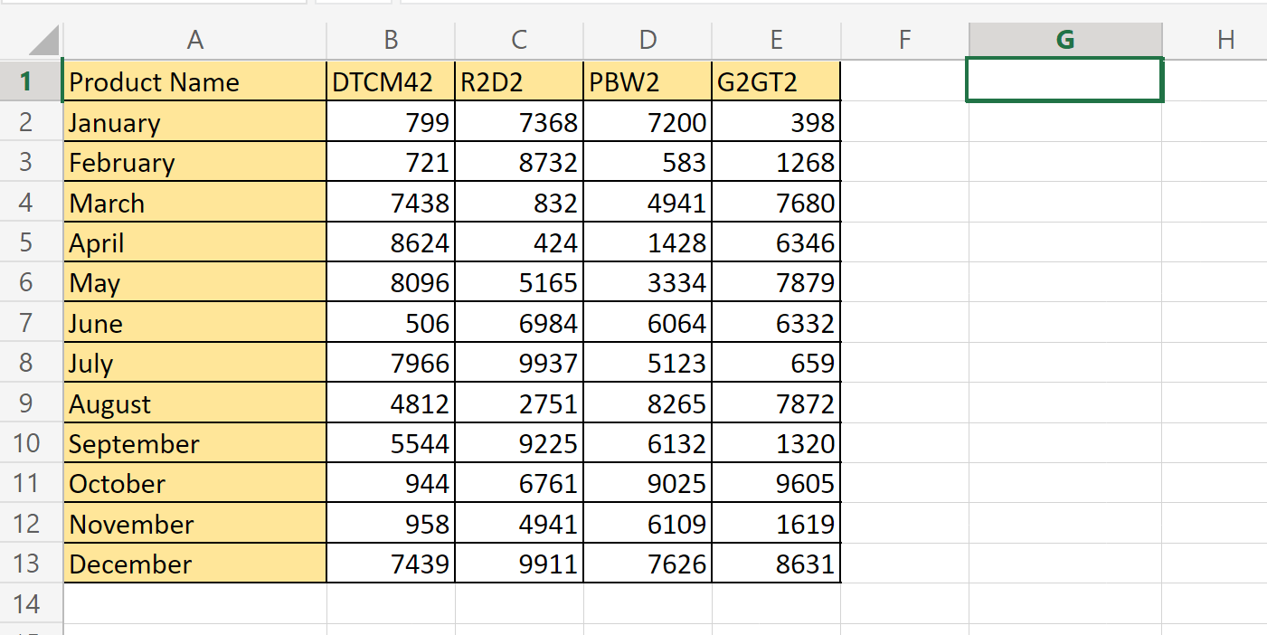
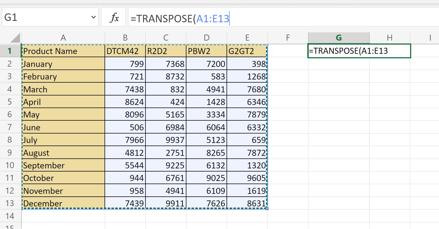
In the example below, we have two tables with the same data. The first table has each row correspond to a different month, while each column corresponds to a product name. The second table is a rotated form of the first table’s data. Each row now corresponds to a product name and each column refers to a month.

To get the values in the second column, we just need to use the following formula in cell G1:
=TRANSPOSE(A1:E13)
The TRANSPOSE function can also be used with other formulas. In the example below we used the FILTER function on the range A2:A6 to get the values less than 30. We then used the TRANSPOSE function to convert the vertical range into a horizontal range.

To get the values in row 8, we used the following formula:
=TRANSPOSE(FILTER(A2:A6,A2:A6<30))
You can make your own copy of the spreadsheet above using the link attached below.
If you’re ready to try out transposing data in Excel, follow our step-by-step guide in the next section!
This guide will show you each step that’s needed to start transposing data in your spreadsheet. You’ll learn how we can use both the Paste Transpose and TRANSPOSE function in Excel to rotate a range.
Follow these steps to start using the Paste Transpose option:
- First, identify which range you would like to transpose. In the example below, we want to transpose the range A1:E13. This means that each column should indicate a month and each row should belong to a particular product name.

- Next, select the entire range that you want to transpose. Type Ctrl + C to copy your selection.

- In another cell in your sheet, right-click and select the Transpose icon under the Paste Options.

- You should now have the transposed range in your spreadsheet. You can now delete the original table if needed.


Next, we’ll show you how you can use the TRANSPOSE function in Microsoft Excel.
- The
TRANSPOSEfunction does not change the original table. Instead, it creates a transposed copy of the source table. In this example, we’ve selected the cell G1 to have ourTRANSPOSEformula.

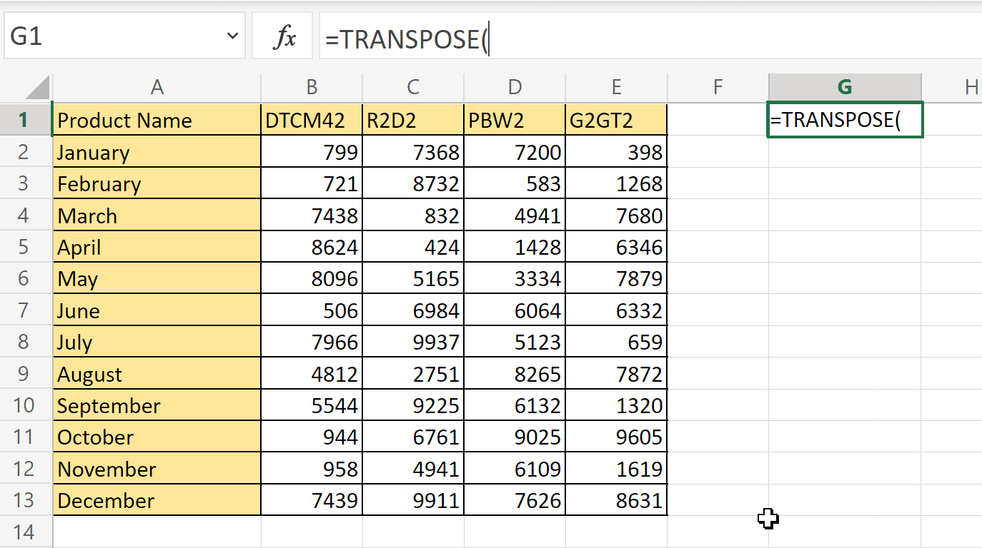
- Next, type out “=TRANSPOSE(“ in the formula bar to begin the function.

- Type in the range you want to transpose as an argument. In this example, we want to transpose the cell range A1:E13.

- Hit the Enter key to return the transposed table.


Frequently Asked Questions (FAQ)
- What happens if my table includes formulas?
If your data includes formulas, Excel will automatically update them to match the new placement of each cell. - Should I transpose my data or use a PivotTable?
Transposing is best used if you only intend to switch two variables as rows and columns.
It’s also better to use a PivotTable if you intend to frequently change the way you want to see your data. PivotTables make it easy for you to select which fields you want to view as either rows or columns.
That’s all you need to remember to start transposing your data in Excel. This step-by-step guide shows how easy it is to rotate a table so that your rows become columns and vice versa.
Transposing tables is just one of many features Excel has to manipulate your spreadsheet. With so many other Excel functions out there, you can surely find one that can help you out.
Are you interested in learning more about what Excel can do? Make sure to subscribe to our newsletter to be the first to know about the latest guides and tutorials from us.

Get emails from us about Excel.
Our goal this year is to create lots of rich, bite-sized tutorials for Excel users like you. If you liked this one, you’d love what we are working on! Readers receive ✨ early access ✨ to new content.

Hi! I’m a Software Developer with a passion for data analytics. Google Sheets has helped me empower my teams to make data-driven decisions. There’s always something new to learn, so let’s explore how you can make life so much easier with spreadsheets!
How to Convert Rows to Columns in Excel?
There are two different methods for converting rows to columns in Excel, which are as follows:
- Method #1 – Transposing Rows to Columns Using Paste Special.
- Method #2 – Transposing Rows to Columns Using TRANSPOSE Formula.
Table of contents
- How to Convert Rows to Columns in Excel?
- #1 Using Paste Special
- Example
- #2 Using TRANSPOSE Formula
- Example
- Advantages
- Disadvantages
- Things to Remember
- Recommended Articles
- #1 Using Paste Special
#1 Using Paste Special
It is an efficient method; it is easy to implement and saves time. Also, this method would be ideal if you want your original formatting to be copied.
You can download this Convert Rows to Columns Excel Template here – Convert Rows to Columns Excel Template
Example
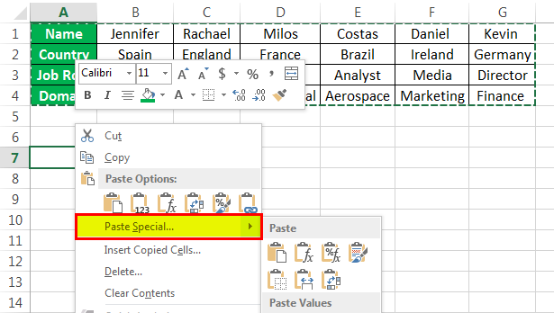
For example, if you have below data of key industry players from various regions, it also shows their job roles as shown in figure1.
| Name | Jennifer | Racheal | Milos | Costas | Daniel | Kevin |
| Country | Spain | England | France | Brazil | Ireland | Germany |
| Job Role | CTO | CEO | Analyst | Analyst | Media | Director |
| Domain | Electronics | Chemical | Mechanical | Aerospace | Marketing | Finance |
In example 1, the players’ names are written in column form. Still, the list becomes too long, and the data entered also seems unorganized. Hence, we would change the rows to columns using paste special methodsPaste special in Excel allows you to paste partial aspects of the data copied. There are several ways to paste special in Excel, including right-clicking on the target cell and selecting paste special, or using a shortcut such as CTRL+ALT+V or ALT+E+S.read more.
The steps to convert rows to columns in Excel using the Paste Special method are as follows:
- Select the whole data which needs to be transformed or transposed. Then, Copy the selected data by simply pressing Ctrl + C keys.

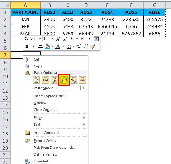
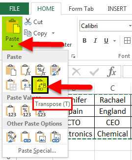
- Select a blank cell and ensure it is outside the original data range. Paste the data by pressing the “Ctrl +V” keys starting at the first blank space or cell. Then, select the down arrow from the toolbar under the “Paste” option and select “Paste Transpose.” But the easy way is to right-click the blank you chose first to paste the data. Then, select “Paste Special” from it.

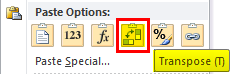
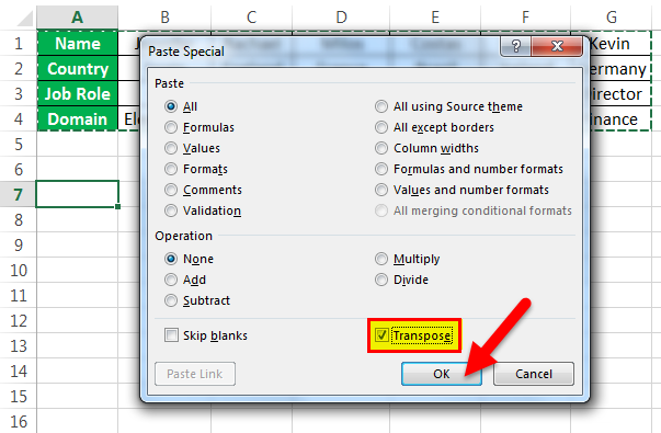
- Then, a “Paste Special” dialog box will appear from which select the “Transpose” option. And click “OK.”

- In the above figure, copy the data which needs to be transposed and then click on the down arrow of the Paste option and form the options select Transpose. (Paste-Transpose)

It shows how the transpose function is performed to convert rows to columns.


#2 Using TRANSPOSE Formula
When a user wants to keep the same connections of the rotating table with the original table, it can use a transposing method using a formula. This method is also quicker in converting rows to columns in Excel. But, it does not keep the source formatting and links it to a transposed table.
Example
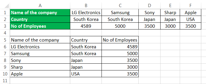
Consider the example below, as shown in figure 6, where it shows the company’s names, location, and the number of employees.
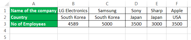
The steps to transpose rows to columns in excel using formula are as follows:
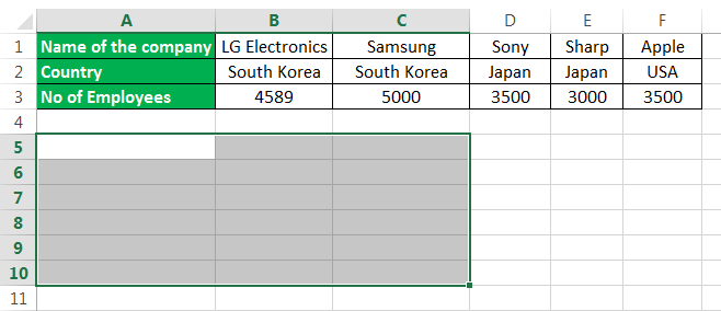
- First, count the number of rows and columns in your original excel table. And then, select the same number of blank cells but ensure you have to transpose the rows to columns to choose the blank cells in the opposite direction. Like in example 2, the number of rows is 3, and the number of columns is 6. So, you will select 6 blank rows and 3 blank columns.
- In the first empty cell, enter the TRANSPOSE formula in excelThe TRANSPOSE function in excel helps rotate (switch) the values from rows to columns and vice versa. Being a part of the Excel lookup and reference functions, its purpose is to organize the data in the desired format. To execute the formula, the exact size of the range to be transposed is selected and the CSE key (“Control+Shift+Enter”) is pressed.
read more ‘=TRANSPOSE($A$1:$F$3)’.
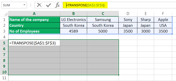
- Since this formula needs to be applied for other blank cells so press ‘Ctrl+Shift+Enter.’
The rows are converted to columns.
Advantages
- The Paste Special method is useful when the user needs the original formatting to be continued.
- In the transpose method, by using the TRANSPOSE function, the converted table will change its data automatically, which means that whenever the user changes the data in the original table, it will automatically change the data in the transposed table, as it is linked to it.
- Converting the rows to columns in Excel sometimes helps the user to make the audience understand their data easily and so that the audience interprets it without much effort.
Disadvantages
- If the number of rows and columns increases, then the transpose method using the Paste Special options cannot perform efficiently. In this case, the “TRANSPOSE” function will be disabled when there are many rows to be converted to columns.
- The “Transpose Paste Special” option does not link the original data to the transposed data. Therefore, if you need to change the data, you must repeat all the steps.
- In the transpose method, the source formatting is not kept the same for the transposed data by using the formula.
- After converting the rows to columns in Excel using a formula, the user cannot edit the data in the transposed table as it is linked to the source data.
Things to Remember
- We can transpose rows to columns using Paste Special methods. We can link the data to the original data by selecting “Paste Link” from the “Paste Special” dialog box.
- We can also use Excel’s INDIRECT formula and ADDRESS functions in ExcelThe address function finds the cell’s address and returns an absolute value. It requires two mandatory arguments: the row number and the column number. For example, if we use =Address(1,2), the result will be $B$1.read more to convert rows to columns and vice-versa.
Recommended Articles
This article is a guide to Convert Rows to Columns in Excel. Here, we discuss switching rows to columns in Excel using the Paste Special and TRANSPOSE formula, practical examples, and a downloadable Excel template. You may learn more about Excel from the following articles: –
- Group Columns in ExcelIn Excel, grouping one or more columns together in a worksheet is referred to as group column and I t allows you to contract or expand the column.read more
- Compare Two Columns in ExcelTwo columns in excel are compared when their entries are studied for similarities and differences.read more
- Use Columns Formula in Excel
- Column Sort in Excel
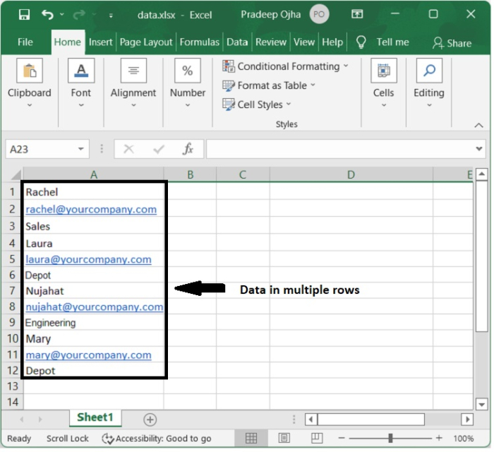
Let’s assume you already have a list of data with many rows that only has one column in an excel sheet, but you want to convert these data to multiple rows and columns, you can achieve this using an Excel formula.
Step 1
Let’s consider the following list of multiple rows data and try to convert those data into multiple columns and rows using excel formula.
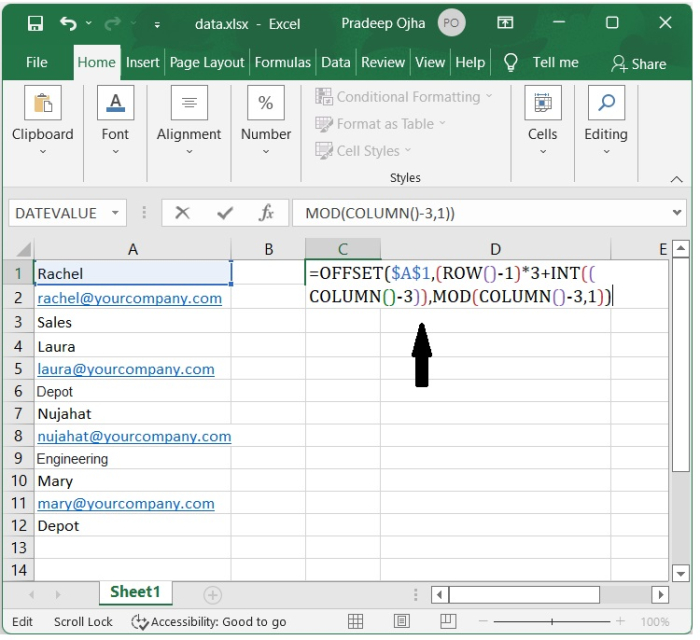
Step 2
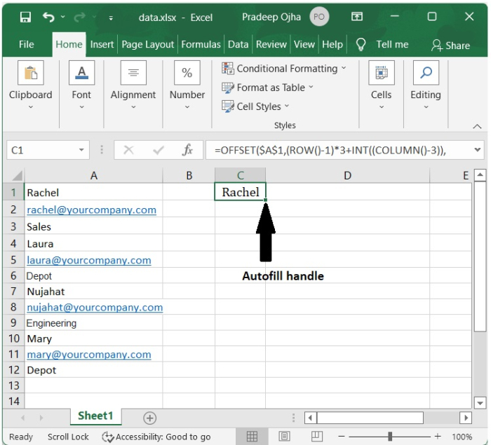
Let’s choose an empty cell (C1) in which we will store the first data of the list of data and type the following formula in cell C1 and press Enter.
=OFFSET($A$1,(ROW()-1)*3+INT((COLUMN()-3)),MOD(COLUMN()-3,1))
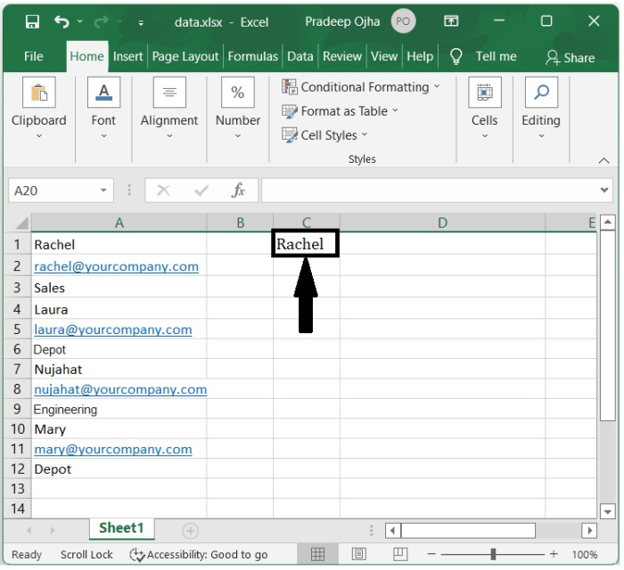
Step 3
Now we get the first-row data of the list data in the cell C1 as shown in the following image.
Step 4
To convert all the list data into multiple columns and rows, we have to simply drag the autofill handle from cell C1.
Step 5
Drag the autofill handle from cell C1 to the right cells as our need, followed by dragging the autofill handle downward to the cells till the value zero is displayed. The data is now displayed in multiple rows and columns as shown in the following screenshot.
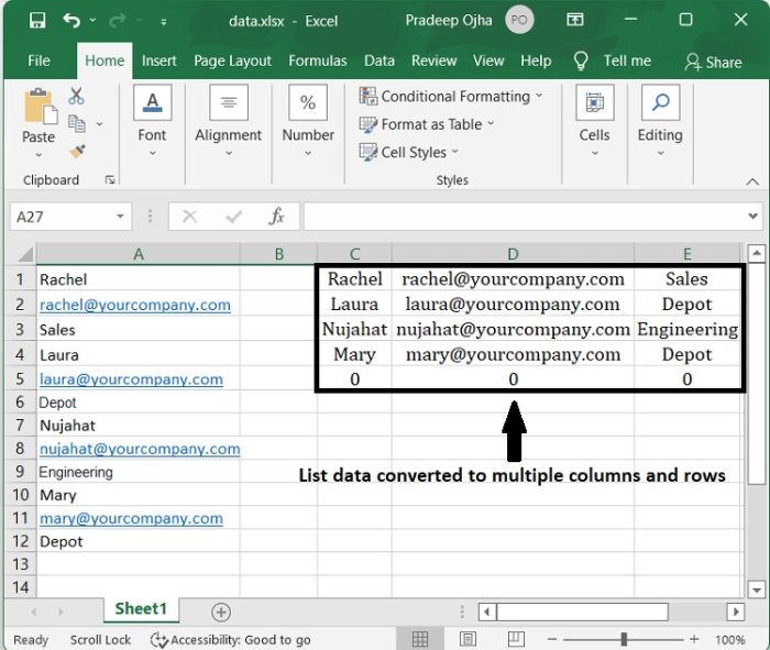
The formula we have used above to convert the list data of multiple rows into multiple columns and rows can be interpreted as follows −
OFFSET($A$1,(ROW()- f_row)*rows_in_set+INT((COLUMN()f_col)/col_in_set), MOD(COLUMN()-f_col,col_in_set))
Where,
-
f_row − row number of this offset formula.
-
f_col − column number of this offset formula.
-
rows_in_set − number of rows that make one record of data from the original data.
-
col_in_set − number of columns of the original list data.
You can change the values of the above fields in the formula according to your list data of multiple rows.
Conclusion
In this tutorial, you learned how to convert list data of multiple rows into multiple columns and rows using a worksheet formula.
Предположим, у вас есть список из одного столбца с несколькими строками, и теперь вы хотите преобразовать этот список в несколько столбцов и строк, как показано ниже, для четкого просмотра данных. Как быстро решить эту проблему в Excel? В этой статье вы можете найти хороший ответ.
Преобразование нескольких строк в столбцы с помощью формулы
Преобразование нескольких строк в столбцы с помощью Kutools for Excel ![]()
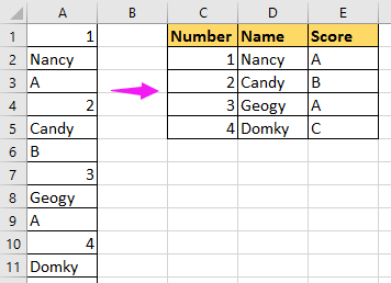
Чтобы преобразовать несколько строк в столбце в несколько столбцов и строк, вы можете использовать формулы, выполнив следующие действия:
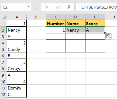
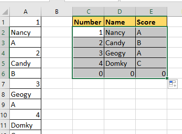
Выберите пустую ячейку, которую вы хотите вывести, поместите первые данные вашего списка, говорит Ячейка C2, и введите эту формулу =OFFSET($A$1,(ROW()-2)*3+INT((COLUMN()-3)),MOD(COLUMN()-3,1)), Затем нажмите Enter , чтобы получить первый список формы данных, затем перетащите дескриптор автозаполнения в нужные ячейки, а затем перетащите дескриптор автозаполнения вниз к ячейкам, пока не отобразится ноль. Смотрите скриншоты:
![]()
Примечание:
Эту формулу можно интерпретировать как
OFFSET ($ A $ 1, (ROW () — f_row) * rows_in_set + INT ((COLUMN () — f_col) / col_in_set), MOD (COLUMN () — f_col, col_in_set))
И в формуле
f_row номер строки этой формулы
f_col это номер столбца этой формулы
rows_in_set это количество строк, которые составляют одну запись данных
col_in_set это количество столбцов исходных данных
Вы можете изменить их по своему усмотрению.
Для некоторых более экологичных формул приведенная выше формула может быть несколько сложной, но не волнуйтесь, Kutools for ExcelАвтора Диапазон транспонирования Утилита может помочь каждому быстро преобразовать несколько строк в столбце в столбцы и строки.
После бесплатная установка Kutools for Excel, пожалуйста, сделайте следующее:
1. Выберите список столбцов и щелкните Кутулс > Диапазон > Диапазон преобразования. Смотрите скриншот:

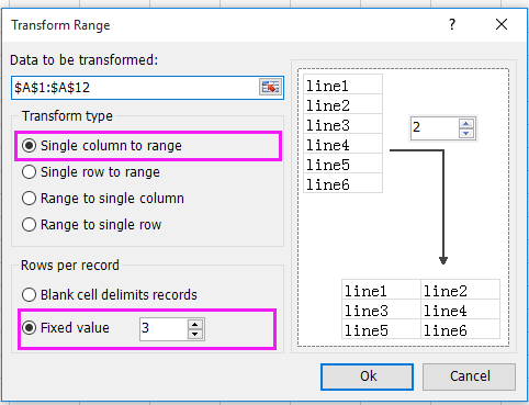
2. Затем в Диапазон транспонирования диалог, проверьте Один столбец для диапазона вариант в Тип трансформации раздел, проверьте Фиксированная стоимость вариант в Строк на запись раздел и введите количество фиксированных столбцов в следующее текстовое поле. Смотрите скриншот:
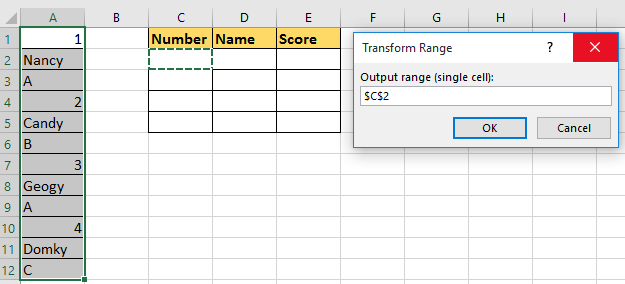
3. Нажмите Ok, и появится диалоговое окно, напоминающее вам о выборе ячейки для вывода результата. Смотрите скриншот:
4. Нажмите OK. И список с несколькими строками был преобразован в несколько столбцов и строк.

Относительные статьи:
- Как массово преобразовать текст в дату в Excel?
- Как преобразовать строчные буквы в правильный или регистр предложений в Excel?
- Как преобразовать время в десятичные часы / минуты / секунды в Excel?
Лучшие инструменты для работы в офисе
Kutools for Excel Решит большинство ваших проблем и повысит вашу производительность на 80%
- Снова использовать: Быстро вставить сложные формулы, диаграммы и все, что вы использовали раньше; Зашифровать ячейки с паролем; Создать список рассылки и отправлять электронные письма …
- Бар Супер Формулы (легко редактировать несколько строк текста и формул); Макет для чтения (легко читать и редактировать большое количество ячеек); Вставить в отфильтрованный диапазон…
- Объединить ячейки / строки / столбцы без потери данных; Разделить содержимое ячеек; Объединить повторяющиеся строки / столбцы… Предотвращение дублирования ячеек; Сравнить диапазоны…
- Выберите Дубликат или Уникальный Ряды; Выбрать пустые строки (все ячейки пустые); Супер находка и нечеткая находка во многих рабочих тетрадях; Случайный выбор …
- Точная копия Несколько ячеек без изменения ссылки на формулу; Автоматическое создание ссылок на несколько листов; Вставить пули, Флажки и многое другое …
- Извлечь текст, Добавить текст, Удалить по позиции, Удалить пробел; Создание и печать промежуточных итогов по страницам; Преобразование содержимого ячеек в комментарии…
- Суперфильтр (сохранять и применять схемы фильтров к другим листам); Расширенная сортировка по месяцам / неделям / дням, периодичности и др .; Специальный фильтр жирным, курсивом …
- Комбинируйте книги и рабочие листы; Объединить таблицы на основе ключевых столбцов; Разделить данные на несколько листов; Пакетное преобразование xls, xlsx и PDF…
- Более 300 мощных функций. Поддерживает Office/Excel 2007-2021 и 365. Поддерживает все языки. Простое развертывание на вашем предприятии или в организации. Полнофункциональная 30-дневная бесплатная пробная версия. 60-дневная гарантия возврата денег.
")
Вкладка Office: интерфейс с вкладками в Office и упрощение работы
- Включение редактирования и чтения с вкладками в Word, Excel, PowerPoint, Издатель, доступ, Visio и проект.
- Открывайте и создавайте несколько документов на новых вкладках одного окна, а не в новых окнах.
- Повышает вашу продуктивность на 50% и сокращает количество щелчков мышью на сотни каждый день!
")
Комментарии (0)
Оценок пока нет. Оцените первым!
See all How-To Articles
This tutorial demonstrates how to transpose rows to columns in Excel and Google Sheets.
Transpose Rows to Columns
In Excel, you can transpose data from rows to columns. This is often used when you copy data from some other application and want to re-organize them to column-oriented. You can transpose rows from a single column, or transpose multiple column rows at once using the Paste special option.
Transpose Rows in One Column
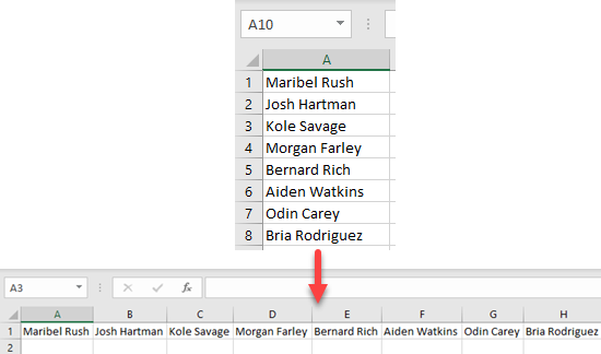
Say you have the following list of names in Column A and want to transpose them to columns in Row 1.
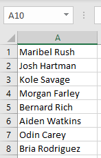
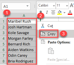
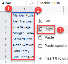
- Select the range to transpose (A1:A8), right-click the selected area, and choose Copy (or use the keyboard shortcut CTRL + C).
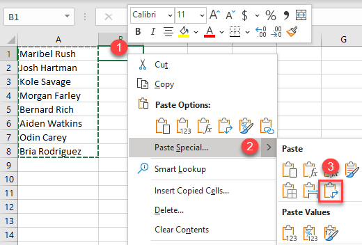
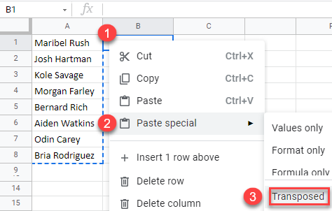
- Right-click the cell where you want to paste transposed data (B1), click the arrow next to Paste Special, and choose the Transpose icon (or use the Transpose shortcut).
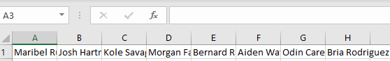
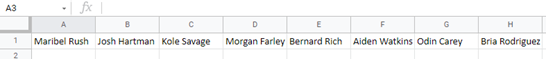
Note: Your paste range can’t intersect with the original, copied range. (That’s why we pasted data in B1, not A1.) After pasting, you can delete the original data in Column A – if not needed – because all values are now in the columns of Row 1.
Transpose Rows in Multiple Columns
You could also have data in rows across multiple columns and need to transpose them. For example, your header is in the first column, but should be in the first row, and each item should have its own row. In the following data set, sales data are organized this way.
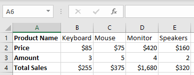
To transpose all rows to columns, follow these steps.
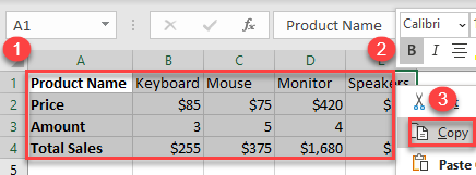
- Select the range to transpose (A1:E4), right-click the selected area, and choose Copy (or use the keyboard shortcut CTRL + C).
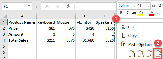
- Right-click the cell where you want to paste transposed data (F1), click the arrow next to Paste Special, and choose the Transpose icon (or use the Transpose shortcut).
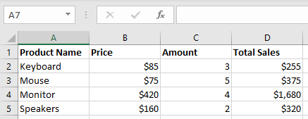
- Now you can delete the original data if you don’t need it since the range is transposed to rows.
Transpose Rows to Columns in Google Sheets
Similar to Excel, you can also transpose rows to columns in Google Sheets.
- Select the range to transpose (A1:A8), right-click the selected area, and choose Copy (or use the keyboard shortcut CTRL + C).
- Right-click the cell where you want to paste transposed data (B1), click Paste Special, and choose Transposed.
As a result, values from Column A are now transposed in Row 1.
Transposing multiple columns works similarly.