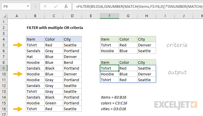
In this example, criteria are entered in the range F5:H6. The logic of the formula is:
item is (tshirt OR hoodie) AND color is (red OR blue) AND city is (denver OR seattle)
The filtering logic of this formula (the include argument) is applied with the ISNUMBER and MATCH functions, together with boolean logic applied in an array operation.
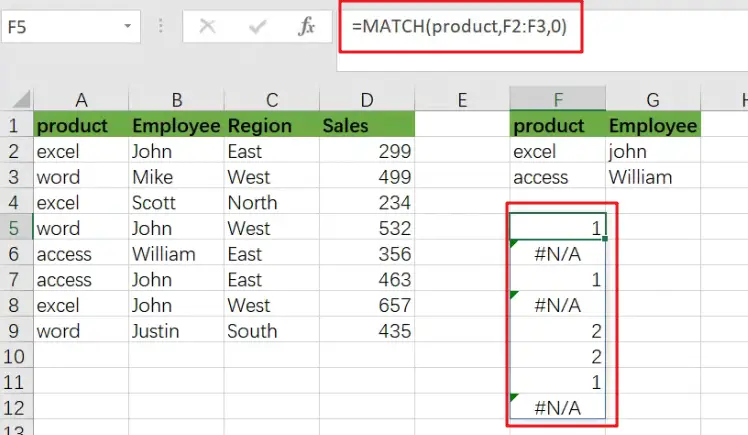
MATCH is configured «backwards», with lookup_values coming from the data, and criteria used for the lookup_array. For example, the first condition is that items must be either a Tshirt or Hoodie. To apply this condition, MATCH is set up like this:
MATCH(items,F5:F6,0) // check for tshirt or hoodie
Because there are 12 values in the data, the result is an array with 12 values like this:
{1;#N/A;#N/A;2;#N/A;2;2;#N/A;1;#N/A;2;1}
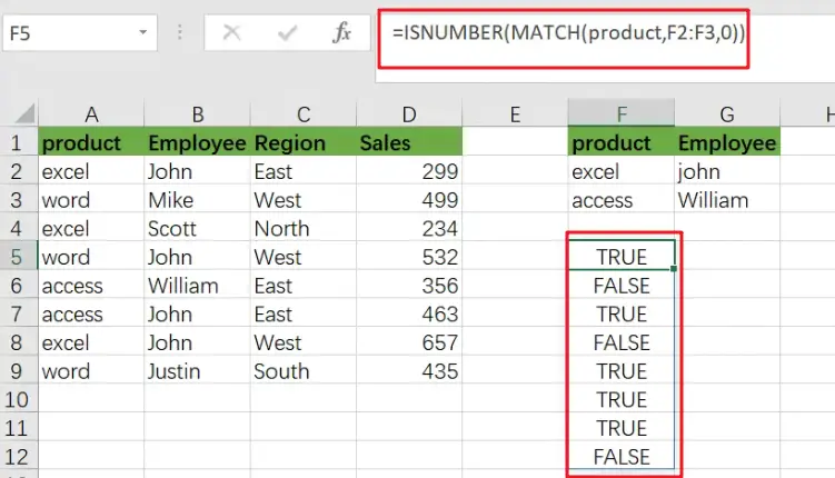
This array contains either #N/A errors (no match) or numbers (match). Notice numbers correspond to items that are either Tshirt or Hoodie. To convert this array into TRUE and FALSE values, the MATCH function is wrapped in the ISNUMBER function:
ISNUMBER(MATCH(items,F5:F6,0))
which yields an array like this:
{TRUE;FALSE;FALSE;TRUE;FALSE;TRUE;TRUE;FALSE;TRUE;FALSE;TRUE;TRUE}
In this array, the TRUE values correspond to tshirt or hoodie.
The full formula contains three expressions like the above used for the include argument of the FILTER function:
ISNUMBER(MATCH(items,F5:F6,0))* // tshirt or hoodie
ISNUMBER(MATCH(colors,G5:G6,0))* // red or blue
ISNUMBER(MATCH(cities,H5:H6,0))) // denver or seattle
After MATCH and ISNUMBER are evaluated, we have three arrays containing TRUE and FALSE values. The math operation of multiplying these arrays together coerces the TRUE and FALSE values to 1s and 0s, so we can visualize the arrays at this point like this:
{1;0;0;1;0;1;1;0;1;0;1;1}*
{1;0;1;1;0;1;0;0;0;0;0;1}*
{1;0;1;0;0;1;0;1;1;0;0;1}
The result, following the rules of boolean arithmetic, is a single array:
{1;0;0;0;0;1;0;0;0;0;0;1}
which becomes the include argument in the FILTER function:
=FILTER(B5:D16,{1;0;0;0;0;1;0;0;0;0;0;1})
The final result is the three rows of data shown in F9:H11
With hard-coded values
Although the formula in the example uses criteria entered directly on the worksheet, criteria can be hard-coded as array constants instead like this:
=FILTER(B5:D16,
ISNUMBER(MATCH(items,{"Tshirt";"Hoodie"},0))*
ISNUMBER(MATCH(colors,{"Red";"Blue"},0))*
ISNUMBER(MATCH(cities,{"Denver";"Seattle"},0)))
Содержание
- FILTER with multiple OR criteria
- Related functions
- Summary
- Explanation
- With hard-coded values
- How to apply multiple filtering criteria by combining AND and OR operations with the FILTER() function in Excel
- Account Information
- Share with Your Friends
- How to apply multiple filtering criteria by combining AND and OR operations with the FILTER() function in Excel
- Must-read Windows coverage
- The operations
- How to use the built-in filter in Excel
- How to use * in Excel
- How to use + in Excel
- And more
- Microsoft Weekly Newsletter
- Filter by using advanced criteria
- Overview of advanced filter criteria
- Sample data
- Comparison operators
- Using the equal sign to type text or a value
- Considering case-sensitivity
- Using pre-defined names
- Creating criteria by using a formula
- Multiple criteria, one column, any criteria true
- Multiple criteria, multiple columns, all criteria true
- Multiple criteria, multiple columns, any criteria true
- Multiple sets of criteria, one column in all sets
- Multiple sets of criteria, multiple columns in each set
- Wildcard criteria
FILTER with multiple OR criteria
Summary
To extract data with multiple OR conditions, you can use the FILTER function together with the MATCH function. In the example shown, the formula in F9 is:
where items (B3:B16), colors (C3:C16), and cities (D3:D16) are named ranges.
This formula returns data where item is (tshirts OR hoodie) AND color is (red OR blue) AND city is (denver OR seattle).
Explanation
In this example, criteria are entered in the range F5:H6. The logic of the formula is:
item is (tshirt OR hoodie) AND color is (red OR blue) AND city is (denver OR seattle)
The filtering logic of this formula (the include argument) is applied with the ISNUMBER and MATCH functions, together with boolean logic applied in an array operation.
MATCH is configured «backwards», with lookup_values coming from the data, and criteria used for the lookup_array. For example, the first condition is that items must be either a Tshirt or Hoodie. To apply this condition, MATCH is set up like this:
Because there are 12 values in the data, the result is an array with 12 values like this:
This array contains either #N/A errors (no match) or numbers (match). Notice numbers correspond to items that are either Tshirt or Hoodie. To convert this array into TRUE and FALSE values, the MATCH function is wrapped in the ISNUMBER function:
which yields an array like this:
In this array, the TRUE values correspond to tshirt or hoodie.
The full formula contains three expressions like the above used for the include argument of the FILTER function:
After MATCH and ISNUMBER are evaluated, we have three arrays containing TRUE and FALSE values. The math operation of multiplying these arrays together coerces the TRUE and FALSE values to 1s and 0s, so we can visualize the arrays at this point like this:
The result, following the rules of boolean arithmetic, is a single array:
which becomes the include argument in the FILTER function:
The final result is the three rows of data shown in F9:H11
With hard-coded values
Although the formula in the example uses criteria entered directly on the worksheet, criteria can be hard-coded as array constants instead like this:
Источник
How to apply multiple filtering criteria by combining AND and OR operations with the FILTER() function in Excel
Account Information
How to apply multiple filtering criteria by combining AND and OR operations with the FILTER() function in Excel
How to apply multiple filtering criteria by combining AND and OR operations with the FILTER() function in Excel
Learn a seemingly tricky way to extract data from your Microsoft Excel spreadsheet.
We may be compensated by vendors who appear on this page through methods such as affiliate links or sponsored partnerships. This may influence how and where their products appear on our site, but vendors cannot pay to influence the content of our reviews. For more info, visit our Terms of Use page.  Image: 200dgr/Shutterstock
Applying multiple criteria against different columns to filter the data set in Microsoft Excel sounds difficult but it really isn’t as hard as it sounds. The most important part is to get the logic between those columns right. For instance, do you want to see all records where one column equals x and another equals y? Or you might want to see all records where one column = x or another column equals y. The results will be very different. In this article, I’ll show you how to include AND and OR operations in Excel’s FILTER() function.
Must-read Windows coverage
In several spots, you’ll read “AND and OR,” which is grammatically awkward. I’m referring to the AND and OR operations generically. We won’t be using the AND() and OR() functions. I’ll use uppercase only to improve readability.
I’m using Microsoft 365 on a Windows 10 64-bit system. The FILTER() function is available in Microsoft 365, Excel Online, Excel 2021, Excel for iPad and iPhone and Excel for Android tablets and phones. I recommend that you wait to upgrade to Windows 11 until all the kinks are worked out. For your convenience, you can download the demonstration .xlsx file.
The operations
The logic operators * and + specify a relationship between the operands in an expression (AND and OR, respectively). Specifically, * (AND) requires that both operands must be true to return true. On the other hand, + (OR) requires that only one operand be true to return true. In our case, operand is a simple expression. For instance
1 + 3 = 4 AND 2 + 1 = 3
returns true while
1 + 3 = 2 AND 2 + 1 = 3
returns false. If we apply the OR operation to the same expressions
1 + 3 = 4 OR 2 + 1 = 3
returns true because at least one expression is true and
1 + 3 = 2 AND 2 + 1 = 3
returns true for the same reason.
Now let’s work through some examples.
How to use the built-in filter in Excel
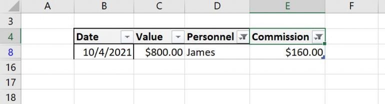
Let’s suppose that you track commissions using the simple data set shown in Figure A. Furthermore, you want to know if anyone is falling below a specific benchmark—say, $200. Fortunately, for users who know how to use the built-in filters, you don’t even need the FILTER() function. However, using the built-in feature works on the source data, and it’s difficult to reference in other expressions, so while it’s easy, it might not be the right solution for every situation.
Figure A
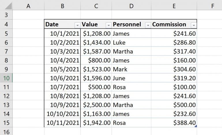 Use the built-in filters.
We have two criteria, personnel and commission. Let’s use a built-in feature to see the filtered set for James with any commission less than or equal to $200, keeping in mind that you must be working with a Table object:
- Click the Personnel dropdown, uncheck (Select All), check James, and click OK. Doing so will display four records.
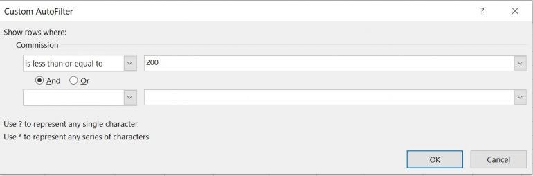
- From the Commission dropdown, choose Number Filters and then choose Less Than Or Equal To, as shown in Figure B.
- Enter 200 in the control to the right of the comparison operator (Figure C) and click OK.
Figure B
 Choose a built-in filter.
Figure C
 Enter the benchmark amount.
As you can see in Figure D, James has only one commission that falls below the $200 benchmark: $160.
Figure D
 The built-in filter feature can handle criteria across multiple columns.
It’s easy but does require a bit of knowledge about how the feature works. On the other hand, the feature works with the data source, and that might not be what you want.
How to use * in Excel
You might have noticed (Figure C) the AND and OR options in the dialog where you entered the benchmark amount. This option allows you to enter other criteria for the same column—Commission. To accomplish an AND across multiple columns, we’ll use the * symbol, which is similar to the AND() function, but AND() doesn’t work as you might expect when combined with FILTER().
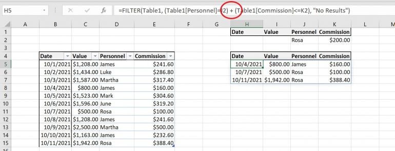
Figure E shows the results of entering the following function
=FILTER(Table1, (Table1[Personnel]=J2) * (Table1[Commission]  Change the name in J2 or the amount in K2 to update the result set.
The * character does a great job of allowing us to apply criteria across multiple rows. But what about OR?
How to use + in Excel
Sometimes, you’ll want to check for the existence of one value or another. When that’s the case, use the + symbol. We can see the difference quickly enough by modifying the function in H5: Replace the * symbol with the + symbol. As you can see in Figure G, there are three records that match the criteria. The personnel value is James, or the commission value is less than or equal to 200.
Figure G
 Three records match the criteria.
And more
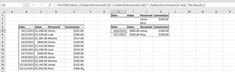
In these simple examples, I worked with only two columns, but it’s no problem to add more. When you do, the parentheses become very important. For example, let’s suppose you want to add another person to the personnel criteria, such as Rosa—you want to match any record where James or Rosa has a commission value less than 200. Again, it’s a simple edit to the original function:
- Select H5.
- Enter (Table1[Personnel]=J3) * between the first and second expressions for the second argument (Figure H). Wrap the first two expression in parentheses: ((Table1[Personnel]=J2) + (Table1[Personnel]=J3)) * (Table1[Commission]
 Modify the function in H5.
 Modify the function in H5.
 Figure I
 This function returns two records.
There are two records for James or Rosa where the commission is less than or equal to 200 (and). To include even more personnel, enter more rows and modify the function by adding a new expression, and remember that entire OR needs to be wrapped in parentheses. The same would be true if you were referencing multiple expressions on the other side. Wrap multiple AND expressions together and wrap multiple OR expressions together.

Microsoft Weekly Newsletter
Be your company’s Microsoft insider by reading these Windows and Office tips, tricks, and cheat sheets.
Источник
Filter by using advanced criteria
If the data you want to filter requires complex criteria (such as Type = «Produce» OR Salesperson = «Davolio»), you can use the Advanced Filter dialog box.
To open the Advanced Filter dialog box, click Data > Advanced.

Salesperson = «Davolio» OR Salesperson = «Buchanan»
Type = «Produce» AND Sales > 1000
Type = «Produce» OR Salesperson = «Buchanan»
(Sales > 6000 AND Sales 3000) OR
(Salesperson = «Buchanan» AND Sales > 1500)
Salesperson = a name with ‘u’ as the second letter
Overview of advanced filter criteria
The Advanced command works differently from the Filter command in several important ways.
It displays the Advanced Filter dialog box instead of the AutoFilter menu.
You type the advanced criteria in a separate criteria range on the worksheet and above the range of cells or table that you want to filter. Microsoft Office Excel uses the separate criteria range in the Advanced Filter dialog box as the source for the advanced criteria.
Sample data
The following sample data is used for all procedures in this article.
The data includes four blank rows above the list range that will be used as a criteria range (A1:C4) and a list range (A6:C10). The criteria range has column labels and includes at least one blank row between the criteria values and the list range.
To work with this data, select it in the following table, copy it, and then paste it in cell A1 of a new Excel worksheet.
Comparison operators
You can compare two values by using the following operators. When two values are compared by using these operators, the result is a logical value—either TRUE or FALSE.
> (greater than sign)
= (greater than or equal to sign)
Greater than or equal to
(not equal to sign)
Using the equal sign to type text or a value
Because the equal sign ( =) is used to indicate a formula when you type text or a value in a cell, Excel evaluates what you type; however, this may cause unexpected filter results. To indicate an equality comparison operator for either text or a value, type the criteria as a string expression in the appropriate cell in the criteria range:
Where entry is the text or value you want to find. For example:
What you type in the cell
What Excel evaluates and displays
Considering case-sensitivity
When filtering text data, Excel doesn’t distinguish between uppercase and lowercase characters. However, you can use a formula to perform a case-sensitive search. For an example, see the section Wildcard criteria.
Using pre-defined names
You can name a range Criteria, and the reference for the range will appear automatically in the Criteria range box. You can also define the name Database for the list range to be filtered and define the name Extract for the area where you want to paste the rows, and these ranges will appear automatically in the List range and Copy to boxes, respectively.
Creating criteria by using a formula
You can use a calculated value that is the result of a formula as your criterion. Remember the following important points:
The formula must evaluate to TRUE or FALSE.
Because you are using a formula, enter the formula as you normally would, and do not type the expression in the following way:
Do not use a column label for criteria labels; either keep the criteria labels blank or use a label that is not a column label in the list range (in the examples that follow, Calculated Average and Exact Match).
If you use a column label in the formula instead of a relative cell reference or a range name, Excel displays an error value such as #NAME? or #VALUE! in the cell that contains the criterion. You can ignore this error because it does not affect how the list range is filtered.
The formula that you use for criteria must use a relative reference to refer to the corresponding cell in the first row of data.
All other references in the formula must be absolute references.
Multiple criteria, one column, any criteria true
Boolean logic: (Salesperson = «Davolio» OR Salesperson = «Buchanan»)
Insert at least three blank rows above the list range that can be used as a criteria range. The criteria range must have column labels. Make sure that there is at least one blank row between the criteria values and the list range.
To find rows that meet multiple criteria for one column, type the criteria directly below each other in separate rows of the criteria range. Using the example, enter:
Click a cell in the list range. Using the example, click any cell in the range A6:C10.
On the Data tab, in the Sort & Filter group, click Advanced.
Do one of the following:
To filter the list range by hiding rows that don’t match your criteria, click Filter the list, in-place.
To filter the list range by copying rows that match your criteria to another area of the worksheet, click Copy to another location, click in the Copy to box, and then click the upper-left corner of the area where you want to paste the rows.
Tip When you copy filtered rows to another location, you can specify which columns to include in the copy operation. Before filtering, copy the column labels for the columns that you want to the first row of the area where you plan to paste the filtered rows. When you filter, enter a reference to the copied column labels in the Copy to box. The copied rows will then include only the columns for which you copied the labels.
In the Criteria range box, enter the reference for the criteria range, including the criteria labels. Using the example, enter $A$1:$C$3.
To move the Advanced Filter dialog box out of the way temporarily while you select the criteria range, click Collapse Dialog  .
.
Using the example, the filtered result for the list range is:
Multiple criteria, multiple columns, all criteria true
Boolean logic: (Type = «Produce» AND Sales > 1000)
Insert at least three blank rows above the list range that can be used as a criteria range. The criteria range must have column labels. Make sure that there is at least one blank row between the criteria values and the list range.
To find rows that meet multiple criteria in multiple columns, type all the criteria in the same row of the criteria range. Using the example, enter:
Click a cell in the list range. Using the example, click any cell in the range A6:C10.
On the Data tab, in the Sort & Filter group, click Advanced.
Do one of the following:
To filter the list range by hiding rows that don’t match your criteria, click Filter the list, in-place.
To filter the list range by copying rows that match your criteria to another area of the worksheet, click Copy to another location, click in the Copy to box, and then click the upper-left corner of the area where you want to paste the rows.
Tip When you copy filtered rows to another location, you can specify which columns to include in the copy operation. Before filtering, copy the column labels for the columns that you want to the first row of the area where you plan to paste the filtered rows. When you filter, enter a reference to the copied column labels in the Copy to box. The copied rows will then include only the columns for which you copied the labels.
In the Criteria range box, enter the reference for the criteria range, including the criteria labels. Using the example, enter $A$1:$C$2.
To move the Advanced Filter dialog box out of the way temporarily while you select the criteria range, click Collapse Dialog .
Using the example, the filtered result for the list range is:
Multiple criteria, multiple columns, any criteria true
Boolean logic: (Type = «Produce» OR Salesperson = «Buchanan»)
Insert at least three blank rows above the list range that can be used as a criteria range. The criteria range must have column labels. Make sure that there is at least one blank row between the criteria values and the list range.
To find rows that meet multiple criteria in multiple columns where any criteria can be true, type the criteria in the different columns and rows of the criteria range. Using the example, enter:
Click a cell in the list range. Using the example, click any cell in the list range A6:C10.
On the Data tab, in the Sort & Filter group, click Advanced.
Do one of the following:
To filter the list range by hiding rows that don’t match your criteria, click Filter the list, in-place.
To filter the list range by copying rows that match your criteria to another area of the worksheet, click Copy to another location, click in the Copy to box, and then click the upper-left corner of the area where you want to paste the rows.
Tip: When you copy filtered rows to another location, you can specify which columns to include in the copy operation. Before filtering, copy the column labels for the columns that you want to the first row of the area where you plan to paste the filtered rows. When you filter, enter a reference to the copied column labels in the Copy to box. The copied rows will then include only the columns for which you copied the labels.
In the Criteria range box, enter the reference for the criteria range, including the criteria labels. Using the example, enter $A$1:$B$3.
To move the Advanced Filter dialog box out of the way temporarily while you select the criteria range, click Collapse Dialog .
Using the example, the filtered result for the list range is:
Multiple sets of criteria, one column in all sets
Boolean logic: ( (Sales > 6000 AND Sales
To find rows that meet multiple sets of criteria where each set includes criteria for one column, include multiple columns with the same column heading. Using the example, enter:
Click a cell in the list range. Using the example, click any cell in the list range A6:C10.
On the Data tab, in the Sort & Filter group, click Advanced.
Do one of the following:
To filter the list range by hiding rows that don’t match your criteria, click Filter the list, in-place.
To filter the list range by copying rows that match your criteria to another area of the worksheet, click Copy to another location, click in the Copy to box, and then click the upper-left corner of the area where you want to paste the rows.
Tip: When you copy filtered rows to another location, you can specify which columns to include in the copy operation. Before filtering, copy the column labels for the columns that you want to the first row of the area where you plan to paste the filtered rows. When you filter, enter a reference to the copied column labels in the Copy to box. The copied rows will then include only the columns for which you copied the labels.
In the Criteria range box, enter the reference for the criteria range, including the criteria labels. Using the example, enter $A$1:$D$3.
To move the Advanced Filter dialog box out of the way temporarily while you select the criteria range, click Collapse Dialog .
Using the example, the filtered result for the list range is:
Multiple sets of criteria, multiple columns in each set
Boolean logic: ( (Salesperson = «Davolio» AND Sales >3000) OR (Salesperson = «Buchanan» AND Sales > 1500) )
Insert at least three blank rows above the list range that can be used as a criteria range. The criteria range must have column labels. Make sure that there is at least one blank row between the criteria values and the list range.
To find rows that meet multiple sets of criteria, where each set includes criteria for multiple columns, type each set of criteria in separate columns and rows. Using the example, enter:
Click a cell in the list range. Using the example, click any cell in the list range A6:C10.
On the Data tab, in the Sort & Filter group, click Advanced.
Do one of the following:
To filter the list range by hiding rows that don’t match your criteria, click Filter the list, in-place.
To filter the list range by copying rows that match your criteria to another area of the worksheet, click Copy to another location, click in the Copy to box, and then click the upper-left corner of the area where you want to paste the rows.
Tip When you copy filtered rows to another location, you can specify which columns to include in the copy operation. Before filtering, copy the column labels for the columns that you want to the first row of the area where you plan to paste the filtered rows. When you filter, enter a reference to the copied column labels in the Copy to box. The copied rows will then include only the columns for which you copied the labels.
In the Criteria range box, enter the reference for the criteria range, including the criteria labels. Using the example, enter $A$1:$C$3.To move the Advanced Filter dialog box out of the way temporarily while you select the criteria range, click Collapse Dialog .
Using the example, the filtered result for the list range would be:
Wildcard criteria
Boolean logic: Salesperson = a name with ‘u’ as the second letter
To find text values that share some characters but not others, do one or more of the following:
Type one or more characters without an equal sign ( =) to find rows with a text value in a column that begin with those characters. For example, if you type the text Dav as a criterion, Excel finds «Davolio,» «David,» and «Davis.»
Use a wildcard character.
Any single character
For example, sm?th finds «smith» and «smyth»
Any number of characters
For example, *east finds «Northeast» and «Southeast»
(tilde) followed by ?, *, or
A question mark, asterisk, or tilde
For example, fy91
Insert at least three blank rows above the list range that can be used as a criteria range. The criteria range must have column labels. Make sure that there is at least one blank row between the criteria values and the list range.
In the rows below the column labels, type the criteria that you want to match. Using the example, enter:
Click a cell in the list range. Using the example, click any cell in the list range A6:C10.
On the Data tab, in the Sort & Filter group, click Advanced.
Do one of the following:
To filter the list range by hiding rows that don’t match your criteria, click Filter the list, in-place
To filter the list range by copying rows that match your criteria to another area of the worksheet, click Copy to another location, click in the Copy to box, and then click the upper-left corner of the area where you want to paste the rows.
Tip: When you copy filtered rows to another location, you can specify which columns to include in the copy operation. Before filtering, copy the column labels for the columns that you want to the first row of the area where you plan to paste the filtered rows. When you filter, enter a reference to the copied column labels in the Copy to box. The copied rows will then include only the columns for which you copied the labels.
In the Criteria range box, enter the reference for the criteria range, including the criteria labels. Using the example, enter $A$1:$B$3.
To move the Advanced Filter dialog box out of the way temporarily while you select the criteria range, click Collapse Dialog .
Using the example, the filtered result for the list range is:
Источник
If you are an valid MS Excel user, you have probably come across a situation where you wanted to filter the data in a separate table with specific criteria. You could do this task manually, which is also acceptable when dealing with a few data items. But if you got an assignment to filter out multiple items from a table consisting of a lot of data along with certain criteria, then doing these kinds of tasks manually would definitely be a stupid decision because this would not only waste your precious time, but you would also get tired of it and won’t complete your task on time.
But don’t be worry about it; for getting out of this fix and filtering out multiple data with specific criteria, all you have to do is read this article carefully.
So let’s dive into it.
Table of Contents
- General formula:
- Syntax Explanation:
- Let’s See How This Formula Works:
- Related Functions
General formula:
The formula below would help you filter out multiple data with specific criteria within a few seconds.
As we have altered the following formula according to the example which we would discuss in this article to understand that how this formula works and how to use this formula:
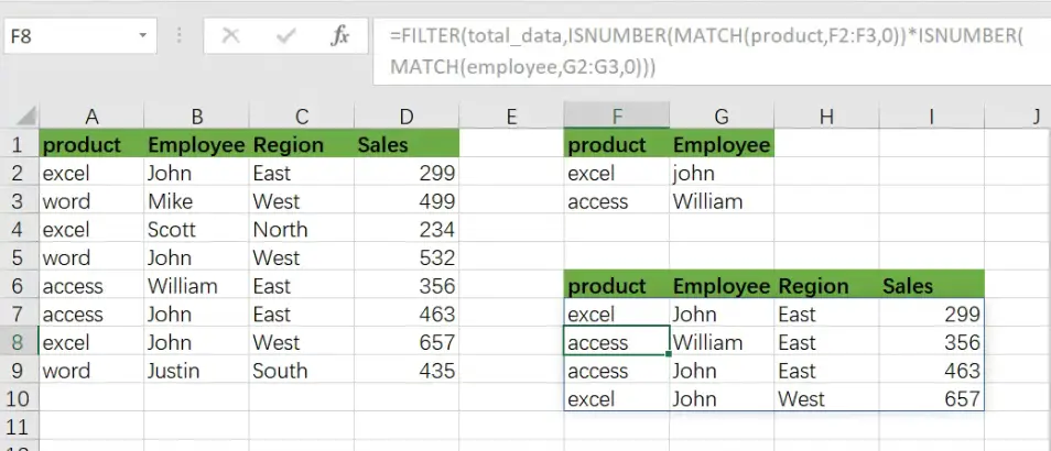
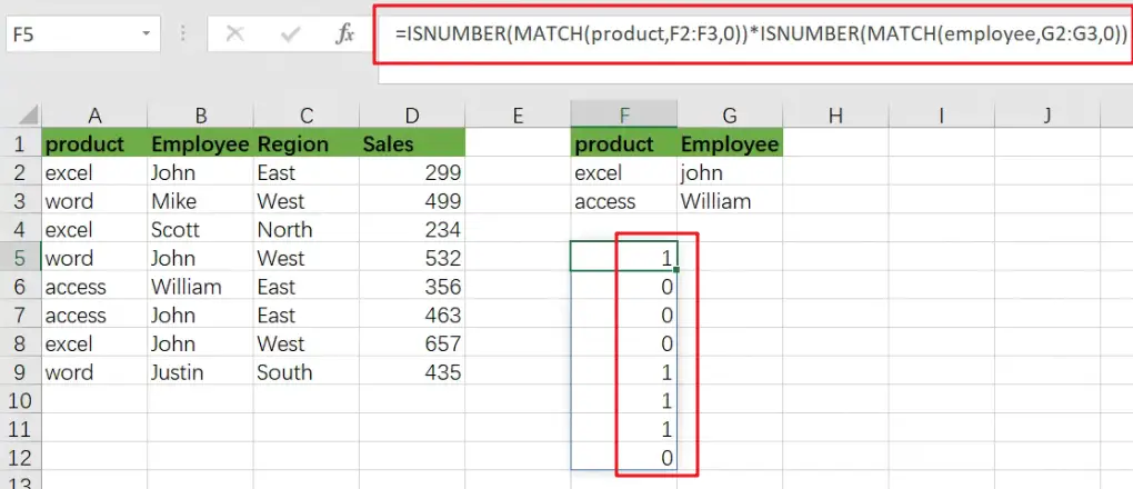
=FILTER(total_data,ISNUMBER(MATCH(product,F2:F3,0))*ISNUMBER(MATCH(employee,G2:G3,0)))
In the formula stated above, we are using the filter function along with the Match function, where ranges are specified for products(A2:A9), employee (B2:B9), and regions (C2:C9).
This formula produces information when the product is “excel” or “access”, AND the employee are “john” or “William”.
Syntax Explanation:
Before we dive into the formula for getting the job done effectively, we need to understand each syntax so that we can know how each syntax helps to Filter with multiple OR criteria :
Filter: This tool helps to narrow down or filter out a variety of data depending on user-defined criteria.Comma symbol(,): In Excel, this symbol functions as a separator and plays a vital role in separating a list of values.Parenthesis(): Its primary role is to group and separate elements.ISNUMBER: The ISNUMBER function determines if a value in a cell or a value derived from another formula is a number. ISNUMBER returns either “true” or “false.”MATCH: The MATCH function looks for a given item in a range of cells and returns the item’s relative location in the range.
Let’s See How This Formula Works:
Criteria for filtering out multiple data are entered in the range F2:G3 in this example. The formula’s rationale is as follows: the product is “excel” or “access”, AND the employee are “john” or “William”.
This formula’s filtering logic (the include parameter) is used with the ISNUMBER and MATCH functions and boolean logic in an array operation.
MATCH is set up “backward,” using lookup values from the data and criteria for the lookup array. For example, the first requirement is that the product be either “excel” or “access”. MATCH is configured as follows to apply this condition:
=MATCH(product,F2:F3,0) // look for excel product
As in the example, there are 8 values in the data; that’s why we get an array with 8 values that looks like the following:
The above array would include #N/A errors (no match) or numbers (match). The numbers on the notice refer to either “excel” or “access” products. To turn this array into TRUE and FALSE values, the MATCH function is wrapped in the ISNUMBER function:
=ISNUMBER(MATCH(product,F2:F3,0))
which results in an array like the following one:
TRUE values in this array match a “excel” or “access”.
The exclusive formula has two expressions similar to the ones used for the FILTER function’s include argument.
Following the evaluation of MATCH and ISNUMBER, we get two arrays containing TRUE and FALSE values. The arithmetic action of multiplying these arrays together converts the TRUE and FALSE values to 1s and 0s.
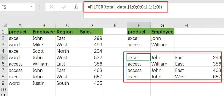
Following the laws of boolean arithmetic, the outcome is a single array which is stated as follows:
which is sent as an argument to the FILTER function like the following:
=FILTER(B5:D16,{1;0;0;0;0;1;0;0;0;0;0;1})
- Excel ISNUMBER function
The Excel ISNUMBER function returns TRUE if the value in a cell is a numeric value, otherwise it will return FALSE.The syntax of the ISNUMBER function is as below:= ISNUMBER (value)… - Excel Filter function
The FILTER function extracts matched records from a collection of data using one or more logical checks. The include argument specifies logical tests, which might encompass a wide variety of formula conditions.==FILTER(array,include,[if empty])… - Excel MATCH function
The Excel MATCH function search a value in an array and returns the position of that item.The MATCH function is a build-in function in Microsoft Excel and it is categorized as a Lookup and Reference Function.The syntax of the MATCH function is as below:= MATCH (lookup_value, lookup_array, [match_type])….
Applying multiple criteria against different columns to filter the data set in Microsoft Excel sounds difficult but it really isn’t as hard as it sounds. The most important part is to get the logic between those columns right. For instance, do you want to see all records where one column equals x and another equals y? Or you might want to see all records where one column = x or another column equals y. The results will be very different. In this article, I’ll show you how to include AND and OR operations in Excel’s FILTER() function.
In several spots, you’ll read “AND and OR,” which is grammatically awkward. I’m referring to the AND and OR operations generically. We won’t be using the AND() and OR() functions. I’ll use uppercase only to improve readability.
SEE: 83 Excel tips every user should master (TechRepublic)
I’m using Microsoft 365 on a Windows 10 64-bit system. The FILTER() function is available in Microsoft 365, Excel Online, Excel 2021, Excel for iPad and iPhone and Excel for Android tablets and phones. I recommend that you wait to upgrade to Windows 11 until all the kinks are worked out. For your convenience, you can download the demonstration .xlsx file.
The operations
The logic operators * and + specify a relationship between the operands in an expression (AND and OR, respectively). Specifically, * (AND) requires that both operands must be true to return true. On the other hand, + (OR) requires that only one operand be true to return true. In our case, operand is a simple expression. For instance
1 + 3 = 4 AND 2 + 1 = 3
returns true while
1 + 3 = 2 AND 2 + 1 = 3
returns false. If we apply the OR operation to the same expressions
1 + 3 = 4 OR 2 + 1 = 3
returns true because at least one expression is true and
1 + 3 = 2 AND 2 + 1 = 3
returns true for the same reason.
Now let’s work through some examples.
How to use the built-in filter in Excel
Let’s suppose that you track commissions using the simple data set shown in Figure A. Furthermore, you want to know if anyone is falling below a specific benchmark—say, $200. Fortunately, for users who know how to use the built-in filters, you don’t even need the FILTER() function. However, using the built-in feature works on the source data, and it’s difficult to reference in other expressions, so while it’s easy, it might not be the right solution for every situation.
Figure A
We have two criteria, personnel and commission. Let’s use a built-in feature to see the filtered set for James with any commission less than or equal to $200, keeping in mind that you must be working with a Table object:
- Click the Personnel dropdown, uncheck (Select All), check James, and click OK. Doing so will display four records.
- From the Commission dropdown, choose Number Filters and then choose Less Than Or Equal To, as shown in Figure B.
- Enter 200 in the control to the right of the comparison operator (Figure C) and click OK.
Figure B
Figure C
As you can see in Figure D, James has only one commission that falls below the $200 benchmark: $160.
Figure D
It’s easy but does require a bit of knowledge about how the feature works. On the other hand, the feature works with the data source, and that might not be what you want.
How to use * in Excel
You might have noticed (Figure C) the AND and OR options in the dialog where you entered the benchmark amount. This option allows you to enter other criteria for the same column—Commission. To accomplish an AND across multiple columns, we’ll use the * symbol, which is similar to the AND() function, but AND() doesn’t work as you might expect when combined with FILTER().
Figure E shows the results of entering the following function
=FILTER(Table1, (Table1[Personnel]=J2) * (Table1[Commission]<=K2), “No Results”)
into H5. At first, nothing happens. That’s because J2 and K2 are empty. Enter James into J2 and 200 into K2. Apply the appropriate formats to the resulting filtered set below if necessary. It’s the one buggy thing I don’t care for—the dynamic array functions ignore formatting. Even after you apply it to the result set (columns H through K), it often disappears when FILTER() recalculates.
Figure E

If you select the different references, your function will look a bit different due to structured referencing. Don’t worry about that; it will still work.
The first argument, Table1, identifies the source data. The second argument
(Table1[Personnel]=J2) * (Table1[Commission]<=K2)
is what we’re interested in. Simply put, the first expression looks for a match to the value in J2 in the Personnel column. With James as the criteria for this column, this expression returns True. The second expression looks for match to the value in K2 in the Commission column, and it too finds a value that it less than or equal to 200, so the expression returns True. Finally, the function returns the data from the rows that both return True. There’s only one, as before.
To check on other personnel, simply change the name in J2. To change the commission benchmark, enter a new value into K2. Keep in mind that the benchmark is always a less than or equal to evaluation because <= is in the function. Figure F shows the result of checking on Rosa’s sales.
Figure F

The * character does a great job of allowing us to apply criteria across multiple rows. But what about OR?
How to use + in Excel
Sometimes, you’ll want to check for the existence of one value or another. When that’s the case, use the + symbol. We can see the difference quickly enough by modifying the function in H5: Replace the * symbol with the + symbol. As you can see in Figure G, there are three records that match the criteria. The personnel value is James, or the commission value is less than or equal to 200.
Figure G
And more
In these simple examples, I worked with only two columns, but it’s no problem to add more. When you do, the parentheses become very important. For example, let’s suppose you want to add another person to the personnel criteria, such as Rosa—you want to match any record where James or Rosa has a commission value less than 200. Again, it’s a simple edit to the original function:
- Select H5.
- Enter (Table1[Personnel]=J3) * between the first and second expressions for the second argument (Figure H). Wrap the first two expression in parentheses: ((Table1[Personnel]=J2) + (Table1[Personnel]=J3)) * (Table1[Commission]<=K2). That extra set of parentheses calculates the OR operation first.
- Enter Rosa in J3 to see the results in Figure I.
Figure H
![]()
Figure I
There are two records for James or Rosa where the commission is less than or equal to 200 (and). To include even more personnel, enter more rows and modify the function by adding a new expression, and remember that entire OR needs to be wrapped in parentheses. The same would be true if you were referencing multiple expressions on the other side. Wrap multiple AND expressions together and wrap multiple OR expressions together.

The FILTER function in Excel is a very useful and frequently used function, that you will likely find the need for in many situations. Note that the FILTER function is only available in Microsoft Office 365, and Microsoft Office Online.
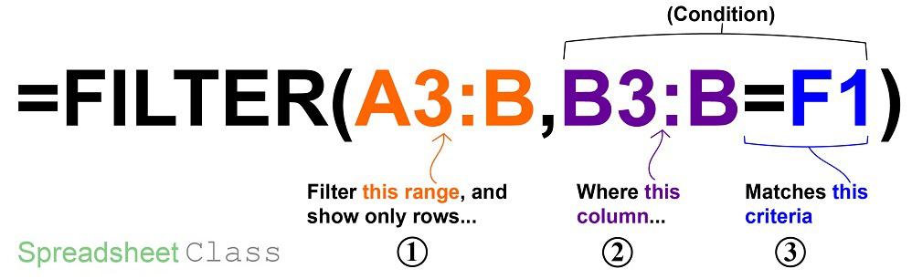
To filter by using the FILTER function in Excel, follow these steps:
- Type =FILTER( to begin your filter formula
- Type the address for the range of cells that contains the data that you want to filter, such as B1:C50
- Type a comma, and then type the condition for the filter, such as C3:C50>3 (To set a condition, first type the address of the «criteria column» such as B1:B, then type an operator symbol such as greater than (>), and then type the criteria, such as the number 3.
- Type a closing parenthesis and then press enter on the keyboard. Your entire formula will look like this: =FILTER(B1:C50,C1:C50>3)
In this article I will start with the basics of using the FILTER function (examples included), and then also show you some more involved ways of using the FILTER function. This article focuses specifically on the FILTER function that is typed into the spreadsheet cells as a formula, and not the filter command available from the toolbar and pop-up menus.
Using the FILTER function in Excel is almost the same as using it in Google Sheets, but there are slight differences between the two. Click here to read the Google Sheets version of this article
Here are the Excel Filters formulas:
Filter by a number
- =FILTER(A3:B12, B3:B12>0.7)
Filter by a cell value
- =FILTER(A3:B12, B3:B12<F1)
Filter by a text string
- =FILTER(A3:B12, B3:B12=»Late»)
Filter where NOT equal to
- =FILTER(A3:E1000, B3:B1000<>»Bob»)
Filter by date
- =FILTER(A3:C12,C3:C12<G1) (Date entered in cell G1)
- =FILTER(A3:C12,C3:C12<DATE(2019,6,1))
Filter by multiple conditions
- =FILTER(A3:C12,(B3:B12=»Late»)*(C3:C12=»Active»)) (AND logic)
- =FILTER(A3:C12, (B3:B12=»Late»)+(C3:C12=»Active»)) (OR logic)
Filter from another sheet
- =FILTER(‘Sheet Name’!A3:B12,’Sheet Name’!B3:B12=»Full Time»)
=FILTER(A3:B12, B3:B12=F1)
(Copy/Paste the formula above into your sheet and modify as needed)
The FILTER function in Excel allows you to filter a range of data by a specified condition, so that a new set of data will be displayed which only shows the rows/columns from the original data set that meets the criteria/condition set in the formula.
Excel description for FILTER function:
Syntax:
=FILTER(array,include,[if_empty])Formula summary: “The FILTER function filters an array based on a Boolean (True/False) array.”
array (Required): The array, or range to filter
include (Required): A Boolean array whose height or width is the same as the array
[if_empty] (Optional): The value to return if all values in the included array are empty (filter returns nothing)
The source range that you want to filter, can be a single column or multiple columns.
The range that is used to check against the criteria that you set, must be a single column (later I will show you how to filter by multiple conditions, but don’t worry about that for now).
The criteria that set in the condition can be manually typed into the formula as a number or text, or it can also be a cell reference.
*Note that the source range and the single column range for the condition, must be the same size (must contain the same number of rows), or the cell will display an error.
Filtering by a single condition in Excel
First let’s go over using the FILTER function in Excel in its simplest form, with a single condition/criteria.
I will show you how to filter by a number, a cell value, a text string, a date… and I will also show you how to use varying «operators» (Less than, Equal to, etc…) in the filter condition.
Part 1: How to filter by a number
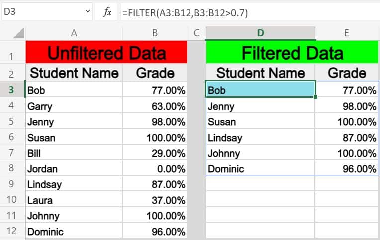
In this first example on how to use the filter function in Excel, the scenario is that we have a list of students and their grades, and that we want to make a filtered list of only students who have a perfect grade.
The task: Show a list of students and their scores, but only those that have a perfect grade
The logic: Filter the range A3:B12, where the column B3:B12 is greater than 0.7 (70%)
The formula: The formula below, is entered in the blue cell (D3), for this example
=FILTER(A3:B12, B3:B12>0.7)
Operators that can be used in the FILTER function:
In this example we are using the operator «=» (Equal To) for the filter condition/criteria, but you can also use any of the following:
«=» (Equals)
«>» (Greater than)
«<» (Less than)
«<>» (Not equal to)
«>=» (Greater than or equal to)
«<=» (Less than or equal to)
Part 2: How to filter by a cell value in Excel
In this example, we want to achieve the same goal as discussed above, but rather than typing the condition that we want to filter by directly into the formula, we are using a cell reference.
When you filter by a cell value in Excel, your sheet will be setup so that you can change the value in the cell at any time, which will automatically update the value that the filter criteria it attached to.
In this example, you will notice that instead of directly typing the number “0.9” into the formula itself, the filter criteria is set as cell G1, where the “0.9” value is entered.
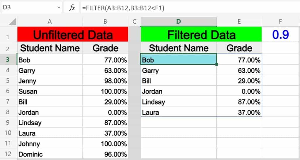
The task: Show a list of students and their scores, but only those that have a score below 90%
The logic: Filter the range A3:B12, where B3:B12 is less than the value that is entered in the cell F1 (0.9)
The formula: The formula below, is entered in the blue cell (D3), for this example
=FILTER(A3:B12, B3:B12<F1)
Part 3: How to filter by text in Excel
In this example, we are going to use a text string as the criteria for the filter formula. This is very similar to using a number, except that you must put the text that you want to filter by inside of quotation marks.
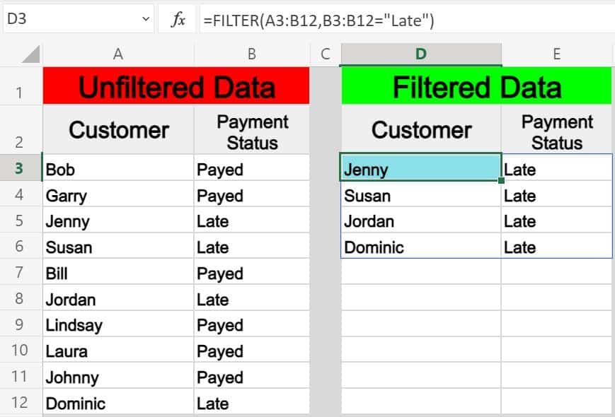
In this scenario we are filtering a list that shows customers and their payment status, and we want to display only customers that have a payment status of “Late”.
The task: Show a list of customers who are past due on their payments
The logic: Filter the range A3:B12, where B3:B12 equals the text, “Late”
The formula: The formula below, is entered in the blue cell (D3), for this example
=FILTER(A3:B12, B3:B12=»Late»)
Part 4: Using NOT EQUAL TO in the Excel FILTER function
Now that you have got a basic understanding of how to use the filter function in Excel, here is another example of filtering by a string of text, but in this example we will use the «not equal» operator (<>), so that you can learn how to filter a range and output data that is NOT equal to criteria that you specify.
In this example we will also use a larger data set to demonstrate a more extensive application of the FILTER function in the real world.
You may be surprised at how often a situation comes up when you need to filter data where it is “not equal to” a certain number or piece of text that you specify.
In this example let’s say that we have a report/spreadsheet that shows data from sales calls that occur at your company, and we want to filter the data so that a specified sales rep (Bob) is NOT included in the filter output.
The task: Show sales call data for all sales reps, except Bob
The logic: Filter the range A2:E1000, where B2:B1000 DOES NOT equal the text, “Bob”
The formula: The formula below, is entered in the blue cell (G3), for this example
=FILTER(A3:E1000, B3:B1000<>»Bob»)
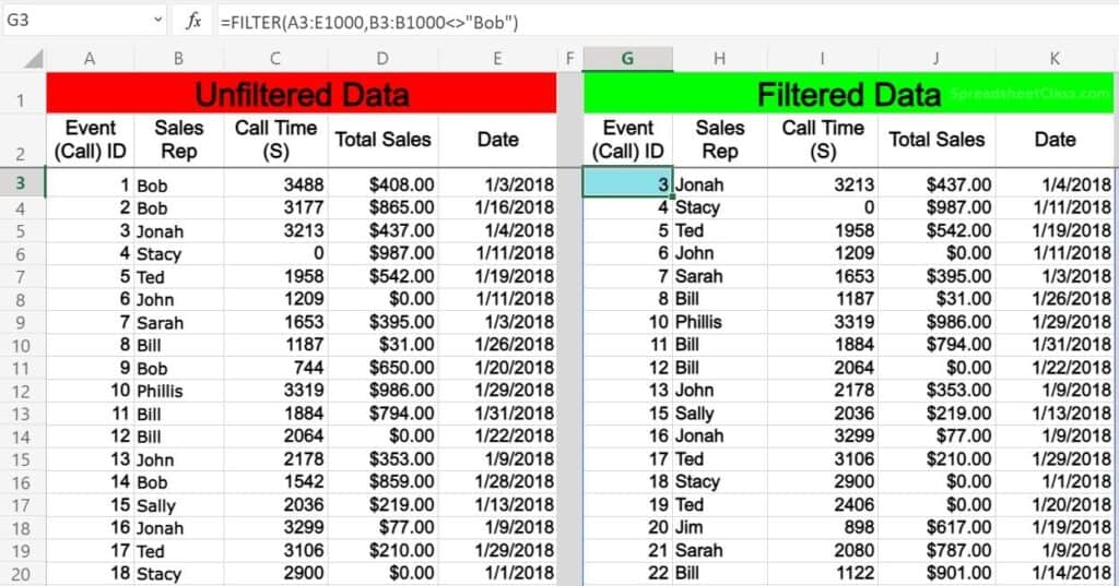
Notice that the filtered data on the right side of the image above does not contain any of the rows/calls that Bob was involved in.
Part 4: How to filter by date in Excel
Filtering by a date in Excel can be done in a couple of ways, which I will show you below. If you try to type a date into the FILTER function like you normally would type into a cell… the formula will not work correctly.
So you can either type the date that you want to filter by into a cell, and then use that cell as a reference in your formula… or you can use the DATE function.
When filtering by date you can use the same operators (>, <, =, etc…) as in other FILTER function applications. In Excel each different day/date is simply a number that is put into a special visual format. For example, in Excel, the date «06/01/2019» is simply the number «43,617», but displayed in date format. When you add one day to the date, this number increments by one each time… i.e «43,618» «43,619» «43,620»
So, one date can be considered to be «greater than» another date, if it is further in the future. Conversely, one date can be said to be «less than» another date, if it is further in the past.
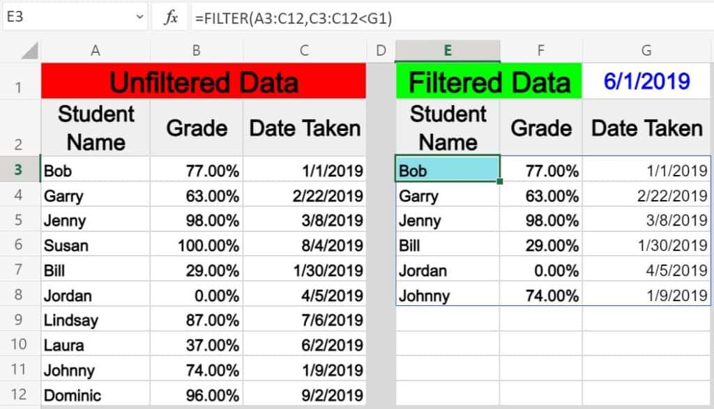
In this first example we will filter by a date by using a cell reference. This is similar to the example we went over in part 2, but in this example instead of working with percentages, we are dealing with dates.
Let’s say that we want to filter a list of students, their test scores, and the dates that the tests were completed… and we want to show only tests that were taken before June (06/01/2019).
Filter by date in Excel example 1:
The task: Show only tests that were taken before June
The logic: Filter the range A3:C12, where C3:C12 is less than the date that is entered in cell G1 (06/01/2019)
The formula: The formula below, is entered in the blue cell (E3), for this example
=FILTER(A3:C12,C3:C12<G1)
Filter by date in Excel example 2:
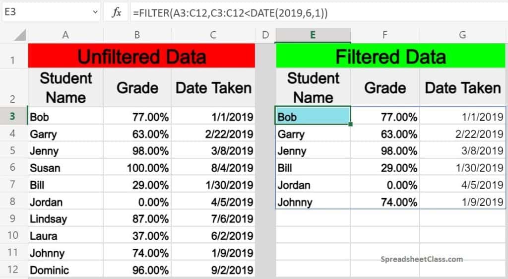
In this second example on filtering by date in Excel we are using the same data as above, and trying to achieve the same results… but instead of using a cell reference, we will use the DATE function so that you can type enter the date directly into the FILTER function.
When using the DATE function to designate a certain date, you must first enter the year, then the month, and then the day… each separated by commas (shown below).
The task: Show only tests that were taken before June
The logic: Filter the range A3:C12, where C3:C12 is less than the date of (06/01/2019)
The formula: The formula below, is entered in the blue cell (E3), for this example
=FILTER(A3:C12,C3:C12<DATE(2019,6,1))
Filter by multiple conditions in Excel
When using the Excel FILTER function you may want to output a set of data that meets more than just one criteria. I will show you two ways to filter by multiple conditions in Excel, depending on the situation that you are in, and depending on how you want to formula to operate.
The normal way of adding another condition to your filter function, (as shown by the formula syntax in Excel), will allow you to set a second condition, where the first AND second condition must be met to be returned in filter output.
However I will also show you how to make a slight modification to the function so that you can choose to set a second condition where EITHER condition can be met to return/display in the filter function’s output/destination. (Separate the conditions with an asterisk to use AND logic, or separate the conditions with a plus sign to use AND logic.)
Part 5: Filtering by 2 conditions where BOTH MUST BE TRUE
In this example, we are going to filter a set of data, and only display rows where BOTH the first condition AND the second condition are met/true.
To use a second condition in this way (with AND logic), simply enter the second condition into the formula after the first condition, separated by an asterisk (*). Each condition must be inside of its own set of parenthesis (shown below).
When using the filter formula with multiple conditions like this, the columns that are referenced in each condition must be different.
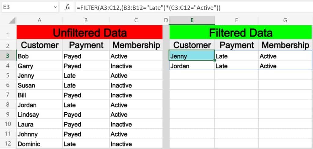
In this scenario we want to filter a list that shows customers, their payment status, and their membership status… and to show only customers who have an active membership AND who are also late on their payment.
This will make sure that customers with an inactive membership who are still designated as being late on payment in the system… are not shown in the filter results, and not put on the list for being sent a «late payment» notice.
The task: Show a list of customers who are late on their payments, but only those with active memberships
The logic: Filter the range A3:C12, where B3:B12 equals the text “Late”, AND where C3:C12 equals the text “Active”
The formula: The formula below, is entered in the blue cell (E3), for this example
=FILTER(A3:C12,(B3:B12=»Late»)*(C3:C12=»Active»))
Part 6: Filtering by 2 conditions where EITHER ARE TRUE, not necessarily both
In this example we are going to filter a set of data and only display rows where EITHER the first condition OR the second condition are met/true.
To use a second condition in this way (with OR logic), simply enter the second condition into the formula after the first condition, separated by a plus sign. Each condition must be inside of its own set of parenthesis (shown below).
When using the FILTER formula in this way, you can choose criteria from the same or different columns.
In this scenario we want to filter the same customer data as shown in the previous example, but this time we want to show a list of customers who EITHER have an active membership OR who are late on their payment. This will give a list of customers who can be sent a notice for payment… including active members, or/also inactive members who are late on their final payment.
The task: Show a list of customers who are active members, and include customers who are late on payment even if they are not active members
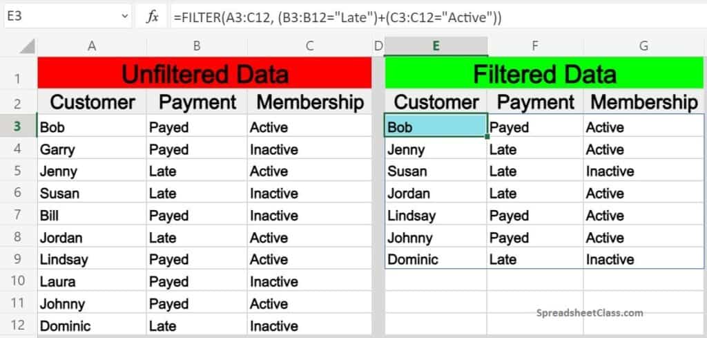
The logic: Filter the range A3:C12, where B3:B12 equals the text “Late”, OR where C3:C12 equals the text “Active”
The formula: The formula below, is entered in the blue cell (E3), for this example
=FILTER(A3:C12, (B3:B12=»Late»)+(C3:C12=»Active»))
How to filter from another sheet in Excel
You may often find situations where you need to filter from another sheet in Excel, where your raw unfiltered data is on one tab, and your filter formula / filter output is on another tab.
This can be done by simply referring to a certain tab name when specifying the ranges in the filter. So where you would normally set a range like «A3:B», when referencing another sheet while filtering you specify the tab name by adding the tab name and an exclamation mark before the column/row portion of the range, like «TabName!A3:B»
However when the tab name has a space in it, it is necessary to use an apostrophe before and after the tab name, like ‘Tab Name’!A3:B.
Here is an example of how to filter data from another tab in Excel, where your filter formula will be on a different tab than the source range.
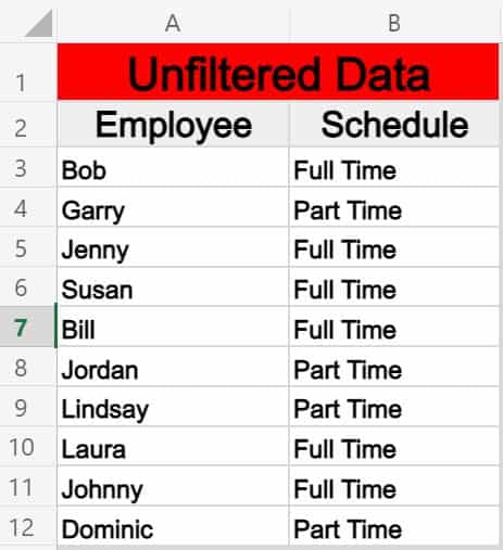
Let’s say that you have a list of employees and their schedule type (Full Time / Part Time) on one tab, and that you want to display a filtered list of full time employees on another tab.
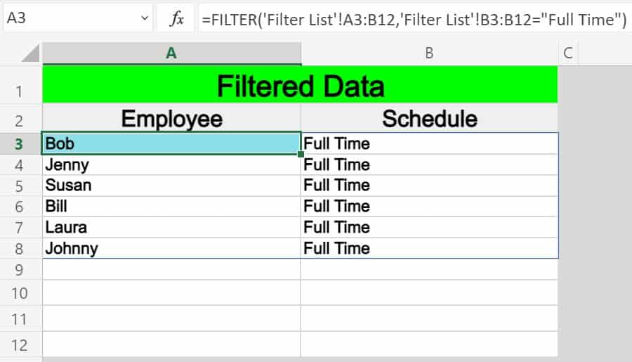
The task: Filter the list of employees on the tab labeled «Filter List», and show a list of employees who have a full time schedule, on a separate tab
The logic: Filter the range ‘Filter List’!A3:B12, where the range ‘Filter List’!B3:B12 is equal to the text «Full Time»
The formula: The formula below, is entered in the blue cell (A3), for this example
=FILTER(‘Filter List’!A3:B12,’Filter List’!B3:B12=»Full Time»)
Here is a list of employees and their schedules, which is held on a tab labeled «Filter List»
And here is a filtered list of employees who have full time schedules, where the filter formula and output data are held on a separate tab.
Pop Quiz: Test your knowledge
Answer the questions below about the Excel FILTER function, to refine your knowledge! Scroll to the very bottom to find the answers to the quiz.
Question #1
Which of the following formulas uses a «cell reference» in the filter condition?
- =FILTER(A1:D15, B1:B15<0.6)
- =FILTER(A2:C15, C2:C15=F1)
- =FILTER(A1:P25, G1:G25=»Yes»)
Question #2
Which of the following formulas uses the «Not Equal» operator?
- =FILTER(C1:T50, J1:J50>100)
- =FILTER(A1:B75, B1:B75=»No»)
- =FILTER(S1:Z100, T1:T100<>»True»)
Question #3
True or False: If the column(s) in the source range and the column in the filter condition are not the same size (if one has more rows than the other), the formula will not work, and will display an error.
- True
- False
Question #4
Which of the following formulas uses AND logic, where BOTH conditions must be met to satisfy the filter criteria?
- =FILTER(C1:F20, (F1:F20=»Yes»)+(E1:E20=»Active»))
- =FILTER(C1:F35, (F1:F35=»Yes»)*(E1:E35=»Active»))
Question #5
Which of the following formulas uses OR logic, where EITHER condition can be met to satisfy the filter criteria?
- =FILTER(A1:K10, (K1:K10=»Yes»)*(J1:J10=»Active»))
- =FILTER(A3:K33, (K3:K33=»Yes»)+(J3:J33=»Active»))
Answers to the questions above:
Question 1: 2
Question 2: 3
Question 3: 1
Question 4: 2
Question 5: 2
If the data you want to filter requires complex criteria (such as Type = «Produce» OR Salesperson = «Davolio»), you can use the Advanced Filter dialog box.
To open the Advanced Filter dialog box, click Data > Advanced.
|
Advanced Filter |
Example |
|---|---|
|
Overview of advanced filter criteria |
|
|
Multiple criteria, one column, any criteria true |
Salesperson = «Davolio» OR Salesperson = «Buchanan» |
|
Multiple criteria, multiple columns, all criteria true |
Type = «Produce» AND Sales > 1000 |
|
Multiple criteria, multiple columns, any criteria true |
Type = «Produce» OR Salesperson = «Buchanan» |
|
Multiple sets of criteria, one column in all sets |
(Sales > 6000 AND Sales < 6500 ) OR (Sales < 500) |
|
Multiple sets of criteria, multiple columns in each set |
(Salesperson = «Davolio» AND Sales >3000) OR |
|
Wildcard criteria |
Salesperson = a name with ‘u’ as the second letter |
Overview of advanced filter criteria
The Advanced command works differently from the Filter command in several important ways.
-
It displays the Advanced Filter dialog box instead of the AutoFilter menu.
-
You type the advanced criteria in a separate criteria range on the worksheet and above the range of cells or table that you want to filter. Microsoft Office Excel uses the separate criteria range in the Advanced Filter dialog box as the source for the advanced criteria.
Sample data
The following sample data is used for all procedures in this article.
The data includes four blank rows above the list range that will be used as a criteria range (A1:C4) and a list range (A6:C10). The criteria range has column labels and includes at least one blank row between the criteria values and the list range.
To work with this data, select it in the following table, copy it, and then paste it in cell A1 of a new Excel worksheet.
|
Type |
Salesperson |
Sales |
|
Type |
Salesperson |
Sales |
|
Beverages |
Suyama |
$5122 |
|
Meat |
Davolio |
$450 |
|
produce |
Buchanan |
$6328 |
|
Produce |
Davolio |
$6544 |
Comparison operators
You can compare two values by using the following operators. When two values are compared by using these operators, the result is a logical value—either TRUE or FALSE.
|
Comparison operator |
Meaning |
Example |
|---|---|---|
|
= (equal sign) |
Equal to |
A1=B1 |
|
> (greater than sign) |
Greater than |
A1>B1 |
|
< (less than sign) |
Less than |
A1<B1 |
|
>= (greater than or equal to sign) |
Greater than or equal to |
A1>=B1 |
|
<= (less than or equal to sign) |
Less than or equal to |
A1<=B1 |
|
<> (not equal to sign) |
Not equal to |
A1<>B1 |
Using the equal sign to type text or a value
Because the equal sign (=) is used to indicate a formula when you type text or a value in a cell, Excel evaluates what you type; however, this may cause unexpected filter results. To indicate an equality comparison operator for either text or a value, type the criteria as a string expression in the appropriate cell in the criteria range:
=»=
entry
»
Where entry is the text or value you want to find. For example:
|
What you type in the cell |
What Excel evaluates and displays |
|---|---|
|
=»=Davolio» |
=Davolio |
|
=»=3000″ |
=3000 |
Considering case-sensitivity
When filtering text data, Excel doesn’t distinguish between uppercase and lowercase characters. However, you can use a formula to perform a case-sensitive search. For an example, see the section Wildcard criteria.
Using pre-defined names
You can name a range Criteria, and the reference for the range will appear automatically in the Criteria range box. You can also define the name Database for the list range to be filtered and define the name Extract for the area where you want to paste the rows, and these ranges will appear automatically in the List range and Copy to boxes, respectively.
Creating criteria by using a formula
You can use a calculated value that is the result of a formula as your criterion. Remember the following important points:
-
The formula must evaluate to TRUE or FALSE.
-
Because you are using a formula, enter the formula as you normally would, and do not type the expression in the following way:
=»=
entry
» -
Do not use a column label for criteria labels; either keep the criteria labels blank or use a label that is not a column label in the list range (in the examples that follow, Calculated Average and Exact Match).
If you use a column label in the formula instead of a relative cell reference or a range name, Excel displays an error value such as #NAME? or #VALUE! in the cell that contains the criterion. You can ignore this error because it does not affect how the list range is filtered.
-
The formula that you use for criteria must use a relative reference to refer to the corresponding cell in the first row of data.
-
All other references in the formula must be absolute references.
Multiple criteria, one column, any criteria true
Boolean logic: (Salesperson = «Davolio» OR Salesperson = «Buchanan»)
-
Insert at least three blank rows above the list range that can be used as a criteria range. The criteria range must have column labels. Make sure that there is at least one blank row between the criteria values and the list range.
-
To find rows that meet multiple criteria for one column, type the criteria directly below each other in separate rows of the criteria range. Using the example, enter:
Type
Salesperson
Sales
=»=Davolio»
=»=Buchanan»
-
Click a cell in the list range. Using the example, click any cell in the range A6:C10.
-
On the Data tab, in the Sort & Filter group, click Advanced.
-
Do one of the following:
-
To filter the list range by hiding rows that don’t match your criteria, click Filter the list, in-place.
-
To filter the list range by copying rows that match your criteria to another area of the worksheet, click Copy to another location, click in the Copy to box, and then click the upper-left corner of the area where you want to paste the rows.
Tip When you copy filtered rows to another location, you can specify which columns to include in the copy operation. Before filtering, copy the column labels for the columns that you want to the first row of the area where you plan to paste the filtered rows. When you filter, enter a reference to the copied column labels in the Copy to box. The copied rows will then include only the columns for which you copied the labels.
-
-
In the Criteria range box, enter the reference for the criteria range, including the criteria labels. Using the example, enter $A$1:$C$3.
To move the Advanced Filter dialog box out of the way temporarily while you select the criteria range, click Collapse Dialog
. -
Using the example, the filtered result for the list range is:
Type
Salesperson
Sales
Meat
Davolio
$450
produce
Buchanan
$6,328
Produce
Davolio
$6,544
Multiple criteria, multiple columns, all criteria true
Boolean logic: (Type = «Produce» AND Sales > 1000)
-
Insert at least three blank rows above the list range that can be used as a criteria range. The criteria range must have column labels. Make sure that there is at least one blank row between the criteria values and the list range.
-
To find rows that meet multiple criteria in multiple columns, type all the criteria in the same row of the criteria range. Using the example, enter:
Type
Salesperson
Sales
=»=Produce»
>1000
-
Click a cell in the list range. Using the example, click any cell in the range A6:C10.
-
On the Data tab, in the Sort & Filter group, click Advanced.
-
Do one of the following:
-
To filter the list range by hiding rows that don’t match your criteria, click Filter the list, in-place.
-
To filter the list range by copying rows that match your criteria to another area of the worksheet, click Copy to another location, click in the Copy to box, and then click the upper-left corner of the area where you want to paste the rows.
Tip When you copy filtered rows to another location, you can specify which columns to include in the copy operation. Before filtering, copy the column labels for the columns that you want to the first row of the area where you plan to paste the filtered rows. When you filter, enter a reference to the copied column labels in the Copy to box. The copied rows will then include only the columns for which you copied the labels.
-
-
In the Criteria range box, enter the reference for the criteria range, including the criteria labels. Using the example, enter $A$1:$C$2.
To move the Advanced Filter dialog box out of the way temporarily while you select the criteria range, click Collapse Dialog
. -
Using the example, the filtered result for the list range is:
Type
Salesperson
Sales
produce
Buchanan
$6,328
Produce
Davolio
$6,544
Multiple criteria, multiple columns, any criteria true
Boolean logic: (Type = «Produce» OR Salesperson = «Buchanan»)
-
Insert at least three blank rows above the list range that can be used as a criteria range. The criteria range must have column labels. Make sure that there is at least one blank row between the criteria values and the list range.
-
To find rows that meet multiple criteria in multiple columns where any criteria can be true, type the criteria in the different columns and rows of the criteria range. Using the example, enter:
Type
Salesperson
Sales
=»=Produce»
=»=Buchanan»
-
Click a cell in the list range. Using the example, click any cell in the list range A6:C10.
-
On the Data tab, in the Sort & Filter group, click Advanced.
-
Do one of the following:
-
To filter the list range by hiding rows that don’t match your criteria, click Filter the list, in-place.
-
To filter the list range by copying rows that match your criteria to another area of the worksheet, click Copy to another location, click in the Copy to box, and then click the upper-left corner of the area where you want to paste the rows.
Tip: When you copy filtered rows to another location, you can specify which columns to include in the copy operation. Before filtering, copy the column labels for the columns that you want to the first row of the area where you plan to paste the filtered rows. When you filter, enter a reference to the copied column labels in the Copy to box. The copied rows will then include only the columns for which you copied the labels.
-
-
In the Criteria range box, enter the reference for the criteria range, including the criteria labels. Using the example, enter $A$1:$B$3.
To move the Advanced Filter dialog box out of the way temporarily while you select the criteria range, click Collapse Dialog
. -
Using the example, the filtered result for the list range is:
Type
Salesperson
Sales
produce
Buchanan
$6,328
Produce
Davolio
$6,544
Multiple sets of criteria, one column in all sets
Boolean logic: ( (Sales > 6000 AND Sales < 6500 ) OR (Sales < 500) )
-
Insert at least three blank rows above the list range that can be used as a criteria range. The criteria range must have column labels. Make sure that there is at least one blank row between the criteria values and the list range.
-
To find rows that meet multiple sets of criteria where each set includes criteria for one column, include multiple columns with the same column heading. Using the example, enter:
Type
Salesperson
Sales
Sales
>6000
<6500
<500
-
Click a cell in the list range. Using the example, click any cell in the list range A6:C10.
-
On the Data tab, in the Sort & Filter group, click Advanced.
-
Do one of the following:
-
To filter the list range by hiding rows that don’t match your criteria, click Filter the list, in-place.
-
To filter the list range by copying rows that match your criteria to another area of the worksheet, click Copy to another location, click in the Copy to box, and then click the upper-left corner of the area where you want to paste the rows.
Tip: When you copy filtered rows to another location, you can specify which columns to include in the copy operation. Before filtering, copy the column labels for the columns that you want to the first row of the area where you plan to paste the filtered rows. When you filter, enter a reference to the copied column labels in the Copy to box. The copied rows will then include only the columns for which you copied the labels.
-
-
In the Criteria range box, enter the reference for the criteria range, including the criteria labels. Using the example, enter $A$1:$D$3.
To move the Advanced Filter dialog box out of the way temporarily while you select the criteria range, click Collapse Dialog
. -
Using the example, the filtered result for the list range is:
Type
Salesperson
Sales
Meat
Davolio
$450
produce
Buchanan
$6,328
Multiple sets of criteria, multiple columns in each set
Boolean logic: ( (Salesperson = «Davolio» AND Sales >3000) OR (Salesperson = «Buchanan» AND Sales > 1500) )
-
Insert at least three blank rows above the list range that can be used as a criteria range. The criteria range must have column labels. Make sure that there is at least one blank row between the criteria values and the list range.
-
To find rows that meet multiple sets of criteria, where each set includes criteria for multiple columns, type each set of criteria in separate columns and rows. Using the example, enter:
Type
Salesperson
Sales
=»=Davolio»
>3000
=»=Buchanan»
>1500
-
Click a cell in the list range. Using the example, click any cell in the list range A6:C10.
-
On the Data tab, in the Sort & Filter group, click Advanced.
-
Do one of the following:
-
To filter the list range by hiding rows that don’t match your criteria, click Filter the list, in-place.
-
To filter the list range by copying rows that match your criteria to another area of the worksheet, click Copy to another location, click in the Copy to box, and then click the upper-left corner of the area where you want to paste the rows.
Tip When you copy filtered rows to another location, you can specify which columns to include in the copy operation. Before filtering, copy the column labels for the columns that you want to the first row of the area where you plan to paste the filtered rows. When you filter, enter a reference to the copied column labels in the Copy to box. The copied rows will then include only the columns for which you copied the labels.
-
-
In the Criteria range box, enter the reference for the criteria range, including the criteria labels. Using the example, enter $A$1:$C$3.To move the Advanced Filter dialog box out of the way temporarily while you select the criteria range, click Collapse Dialog
. -
Using the example, the filtered result for the list range would be:
Type
Salesperson
Sales
produce
Buchanan
$6,328
Produce
Davolio
$6,544
Wildcard criteria
Boolean logic: Salesperson = a name with ‘u’ as the second letter
-
To find text values that share some characters but not others, do one or more of the following:
-
Type one or more characters without an equal sign (=) to find rows with a text value in a column that begin with those characters. For example, if you type the text Dav as a criterion, Excel finds «Davolio,» «David,» and «Davis.»
-
Use a wildcard character.
Use
To find
? (question mark)
Any single character
For example, sm?th finds «smith» and «smyth»* (asterisk)
Any number of characters
For example, *east finds «Northeast» and «Southeast»~ (tilde) followed by ?, *, or ~
A question mark, asterisk, or tilde
For example, fy91~? finds «fy91?»
-
-
Insert at least three blank rows above the list range that can be used as a criteria range. The criteria range must have column labels. Make sure that there is at least one blank row between the criteria values and the list range.
-
In the rows below the column labels, type the criteria that you want to match. Using the example, enter:
Type
Salesperson
Sales
=»=Me*»
=»=?u*»
-
Click a cell in the list range. Using the example, click any cell in the list range A6:C10.
-
On the Data tab, in the Sort & Filter group, click Advanced.
-
Do one of the following:
-
To filter the list range by hiding rows that don’t match your criteria, click Filter the list, in-place
-
To filter the list range by copying rows that match your criteria to another area of the worksheet, click Copy to another location, click in the Copy to box, and then click the upper-left corner of the area where you want to paste the rows.
Tip: When you copy filtered rows to another location, you can specify which columns to include in the copy operation. Before filtering, copy the column labels for the columns that you want to the first row of the area where you plan to paste the filtered rows. When you filter, enter a reference to the copied column labels in the Copy to box. The copied rows will then include only the columns for which you copied the labels.
-
-
In the Criteria range box, enter the reference for the criteria range, including the criteria labels. Using the example, enter $A$1:$B$3.
To move the Advanced Filter dialog box out of the way temporarily while you select the criteria range, click Collapse Dialog
. -
Using the example, the filtered result for the list range is:
Type
Salesperson
Sales
Beverages
Suyama
$5,122
Meat
Davolio
$450
produce
Buchanan
$6,328
Need more help?
You can always ask an expert in the Excel Tech Community or get support in the Answers community.
I am trying to filter for multiple criteria, but I see that the «Filter» option only has 2 fields for «AND/OR» options. I have a column full of links. I want to extract all rows that contain these in it:
.pdf
.doc
.docx
.xls
.xlsx
.rtf
.txt
.csv
.pps
Is there a good way to do this?
asked Aug 19, 2010 at 14:14
![]()
The regular filter options in Excel don’t allow for more than 2 criteria settings. To do 2+ criteria settings, you need to use the Advanced Filter option. Below are the steps I did to try this out.
http://www.bettersolutions.com/excel/EDZ483/QT419412321.htm
Set up the criteria. I put this above the values I want to filter. You could do that or put on a different worksheet. Note that putting the criteria in rows will make it an ‘OR’ filter and putting them in columns will make it an ‘AND’ filter.
- E1 : Letters
- E2 : =m
- E3 : =h
- E4 : =j
I put the data starting on row 5:
- A5 : Letters
- A6 :
- A7 :
- …
Select the first data row (A6) and click the Advanced Filter option. The List Range should be pre-populated. Select the Criteria range as E1:E4 and click OK.
That should be it. Note that I use the ‘=’ operator. You will want to use something a bit different to test for file extensions.
answered Aug 19, 2010 at 20:24
![]()
Edward LenoEdward Leno
6,2073 gold badges33 silver badges49 bronze badges
Maybe not as elegant but another possibility would be to write a formula to do the check and fill it in an adjacent column. You could then filter on that column.
The following looks in cell b14 and would return true for all the file types you mention. This assumes that the file extension is by itself in the column. If it’s not it would be a little more complicated but you could still do it this way.
=OR(B14=".pdf",B14=".doc",B14=".docx",B14=".xls",B14=".xlsx",B14=".rtf",B14=".txt",B14=".csv",B14=".pps")
Like I said, not as elegant as the advanced filters but options are always good.
answered Mar 19, 2011 at 0:25
![]()
Justin OhmsJustin Ohms
3,20930 silver badges44 bronze badges
You can pass an array as the first AutoFilter argument and use the xlFilterValues operator.
This will display PDF, DOC and DOCX filetypes.
Criteria1:=Array(".pdf", ".doc", ".docx"), Operator:=xlFilterValues
answered Mar 5, 2013 at 1:00
![]()
JoshuaJoshua
3572 silver badges5 bronze badges
0
This tutorial demonstrates the capabilities of advanced filters in Excel.
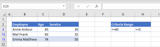
AutoFilter
Excel enables you to filter data by using its efficient Filter tool on the Ribbon or the FILTER Function (in newer versions of Excel). Many find these features very useful.
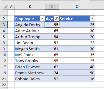
However, the filter tool has some very specific limitations. You can filter using AND logic in a single column – so you can filter everyone who is older than 50 and whose years of service is greater than 20. Then, if you wish to filter on a second column, (service) the data has to be contained within the first filter (age).
In the graphic above, you have filtered on age (greater than 50). You can now filter once again on service, but only the service within the already filtered age criteria are available to filter on. If you then clear the filter, you can see that there is data in the service column ranging from 2 to 50. There are several ways you can filter, but some ways you cannot.
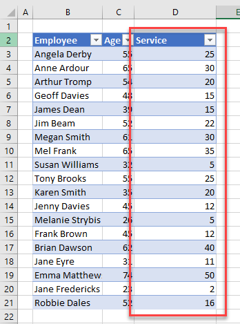
For example, you can use OR logic in a single column by filtering on multiple values in that column.
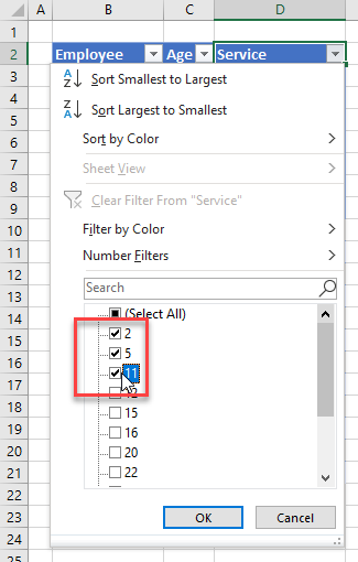
In the example above, the data is filtered to only show rows where years of service is 2, 5, or 11.
- To use a greater than / less than amount, use the number filter option. Select the drop down next to the heading you wish to filter. Then click Number Filters and select the relevant option – in this instance, Greater Than.
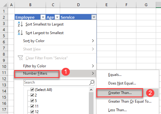
- Type in the comparison value and click OK.
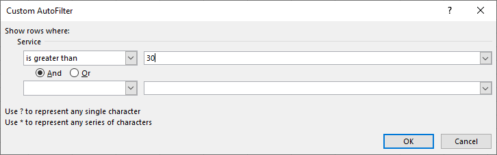
This shows all rows where years of service is greater than 30.
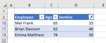
You can also use the And / Or options available in Custom AutoFilter.
The filter below returns all records where years of service is between 20 and 30 years – greater than 20 And less than 30.
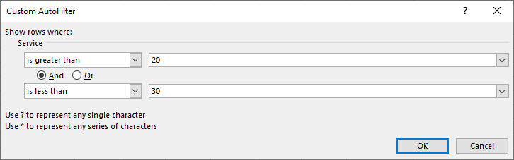
Whereas this one returns all records that are up to 20 Or over 30.
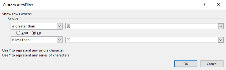
However, should you want to filter all the records where the service is greater than 20 or the age is greater than 50, you would not be able to use AutoFilter to do so.
Advanced Data Filter
Advanced Filter in Excel lets you set a criteria range that enables you to filter on two or more columns of data using and/or scenarios (“Filter With Multiple Criteria” example below). But first, note that it’s also a great way to extract unique data from a list with duplicates.
Extract Unique List
Excel now has a feature that enables you to remove duplicates and quickly isolate unique records. But this feature is relatively new, so alternatively, you can use advanced filters to remove duplicates in any version.
Consider the data below. Somehow, you have managed to end up with duplicates in your data. (Perhaps the entries were copy-pasted from overlapping sources.) You need to remove the duplicates to clean up and use the dataset.
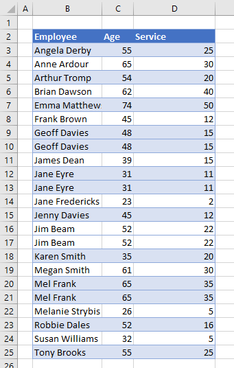
- Highlight the data, and then in the Ribbon, select Data > Sort & Filter > Advanced.
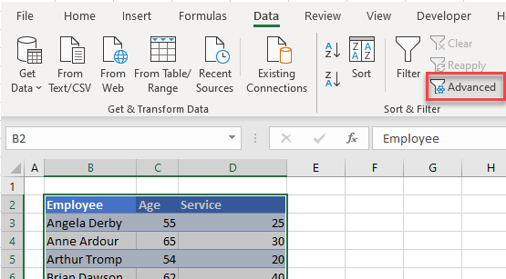
- In the Advanced Filter dialog, select the following:
- Action: Copy to another Location.
- List Range: Should already be selected – what you have highlighted.
- Criteria Range: This should be any blank cell.
- Copy To: A blank area of the worksheet.
- Unique records only: Make sure this is checked.
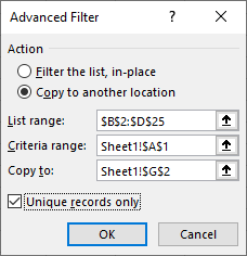
- Click OK to extract unique records.
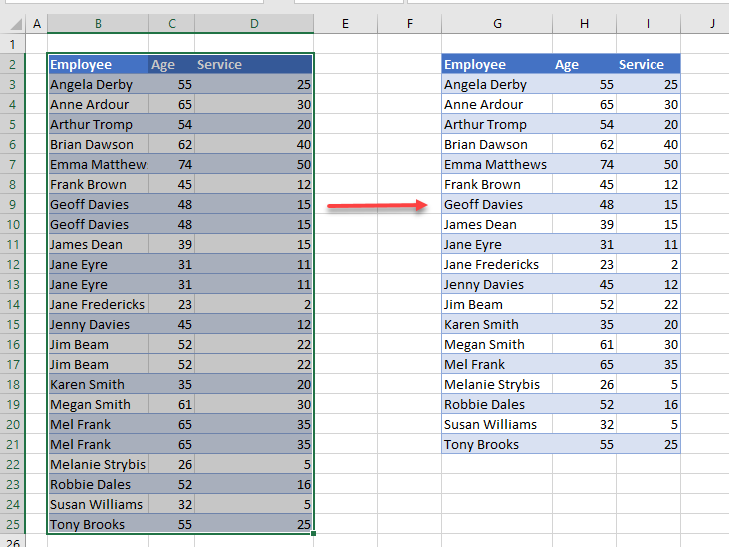
Filter With Multiple Criteria
To filter data on multiple columns with an AND scenario, set up a criteria table for the data filter. In the graphic below, you wish to find all employees who are over 65 and have had over 5 years of service.
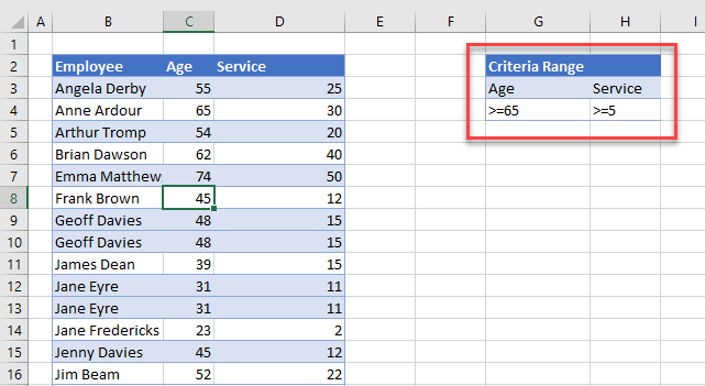
Now, you can do this using AutoFilter, but let’s use advanced filters here.
- In the Data menu, select Sort & Filter > Advanced.
- Then, in the Advanced Filter dialog box, select these options:
- Action: Select Filter the list, in-place.
- List Range: your selected data (e.g., B2:D25 – including headings!).
- Criteria range: make sure you have selected the headings and the values (e.g., G3:G4 as shown in the graphic below).
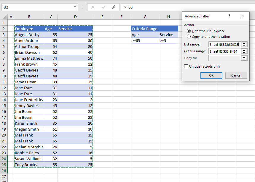
- Click OK to filter the data.
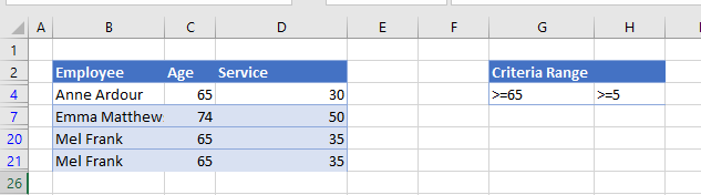
Now, let’s try an OR filter:

This criteria statement finds all employees who are 65 or older, or who have worked at the firm for at least 20 years.
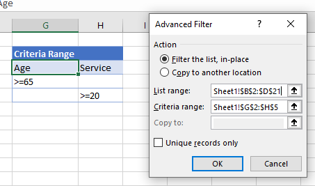
Expand your criteria to include the extra row, and then click OK.
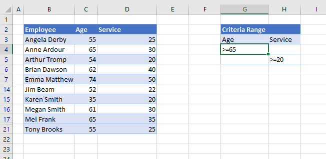
Create Multiple Criteria Scenarios
You can further expand your criteria to include multiple scenarios.
For this example, select all employees who are:
- 65 and over, or
- 60 or over and have worked for the firm for more than 5 years, or
- 55 or over and have worked for the firm for more than 10 years, or
- 50 or over and have worked for the firm for more than 20 years.
The criteria range should be set up thusly:
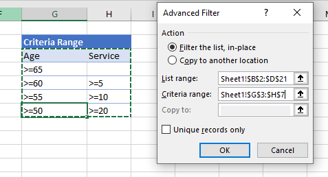
Click OK to implement the filters.