
The IF function allows you to make a logical comparison between a value and what you expect by testing for a condition and returning a result if True or False.
-
=IF(Something is True, then do something, otherwise do something else)
So an IF statement can have two results. The first result is if your comparison is True, the second if your comparison is False.
IF statements are incredibly robust, and form the basis of many spreadsheet models, but they are also the root cause of many spreadsheet issues. Ideally, an IF statement should apply to minimal conditions, such as Male/Female, Yes/No/Maybe, to name a few, but sometimes you might need to evaluate more complex scenarios that require nesting* more than 3 IF functions together.
* “Nesting” refers to the practice of joining multiple functions together in one formula.
Use the IF function, one of the logical functions, to return one value if a condition is true and another value if it’s false.
Syntax
IF(logical_test, value_if_true, [value_if_false])
For example:
-
=IF(A2>B2,»Over Budget»,»OK»)
-
=IF(A2=B2,B4-A4,»»)
|
Argument name |
Description |
|
logical_test (required) |
The condition you want to test. |
|
value_if_true (required) |
The value that you want returned if the result of logical_test is TRUE. |
|
value_if_false (optional) |
The value that you want returned if the result of logical_test is FALSE. |
Remarks
While Excel will allow you to nest up to 64 different IF functions, it’s not at all advisable to do so. Why?
-
Multiple IF statements require a great deal of thought to build correctly and make sure that their logic can calculate correctly through each condition all the way to the end. If you don’t nest your formula 100% accurately, then it might work 75% of the time, but return unexpected results 25% of the time. Unfortunately, the odds of you catching the 25% are slim.
-
Multiple IF statements can become incredibly difficult to maintain, especially when you come back some time later and try to figure out what you, or worse someone else, was trying to do.
If you find yourself with an IF statement that just seems to keep growing with no end in sight, it’s time to put down the mouse and rethink your strategy.
Let’s look at how to properly create a complex nested IF statement using multiple IFs, and when to recognize that it’s time to use another tool in your Excel arsenal.
Examples
Following is an example of a relatively standard nested IF statement to convert student test scores to their letter grade equivalent.

-
=IF(D2>89,»A»,IF(D2>79,»B»,IF(D2>69,»C»,IF(D2>59,»D»,»F»))))
This complex nested IF statement follows a straightforward logic:
-
If the Test Score (in cell D2) is greater than 89, then the student gets an A
-
If the Test Score is greater than 79, then the student gets a B
-
If the Test Score is greater than 69, then the student gets a C
-
If the Test Score is greater than 59, then the student gets a D
-
Otherwise the student gets an F
This particular example is relatively safe because it’s not likely that the correlation between test scores and letter grades will change, so it won’t require much maintenance. But here’s a thought – what if you need to segment the grades between A+, A and A- (and so on)? Now your four condition IF statement needs to be rewritten to have 12 conditions! Here’s what your formula would look like now:
-
=IF(B2>97,»A+»,IF(B2>93,»A»,IF(B2>89,»A-«,IF(B2>87,»B+»,IF(B2>83,»B»,IF(B2>79,»B-«, IF(B2>77,»C+»,IF(B2>73,»C»,IF(B2>69,»C-«,IF(B2>57,»D+»,IF(B2>53,»D»,IF(B2>49,»D-«,»F»))))))))))))
It’s still functionally accurate and will work as expected, but it takes a long time to write and longer to test to make sure it does what you want. Another glaring issue is that you’ve had to enter the scores and equivalent letter grades by hand. What are the odds that you’ll accidentally have a typo? Now imagine trying to do this 64 times with more complex conditions! Sure, it’s possible, but do you really want to subject yourself to this kind of effort and probable errors that will be really hard to spot?
Tip: Every function in Excel requires an opening and closing parenthesis (). Excel will try to help you figure out what goes where by coloring different parts of your formula when you’re editing it. For instance, if you were to edit the above formula, as you move the cursor past each of the ending parentheses “)”, its corresponding opening parenthesis will turn the same color. This can be especially useful in complex nested formulas when you’re trying to figure out if you have enough matching parentheses.
Additional examples
Following is a very common example of calculating Sales Commission based on levels of Revenue achievement.

-
=IF(C9>15000,20%,IF(C9>12500,17.5%,IF(C9>10000,15%,IF(C9>7500,12.5%,IF(C9>5000,10%,0)))))
This formula says IF(C9 is Greater Than 15,000 then return 20%, IF(C9 is Greater Than 12,500 then return 17.5%, and so on…
While it’s remarkably similar to the earlier Grades example, this formula is a great example of how difficult it can be to maintain large IF statements – what would you need to do if your organization decided to add new compensation levels and possibly even change the existing dollar or percentage values? You’d have a lot of work on your hands!
Tip: You can insert line breaks in the formula bar to make long formulas easier to read. Just press ALT+ENTER before the text you want to wrap to a new line.
Here is an example of the commission scenario with the logic out of order:

Can you see what’s wrong? Compare the order of the Revenue comparisons to the previous example. Which way is this one going? That’s right, it’s going from bottom up ($5,000 to $15,000), not the other way around. But why should that be such a big deal? It’s a big deal because the formula can’t pass the first evaluation for any value over $5,000. Let’s say you’ve got $12,500 in revenue – the IF statement will return 10% because it is greater than $5,000, and it will stop there. This can be incredibly problematic because in a lot of situations these types of errors go unnoticed until they’ve had a negative impact. So knowing that there are some serious pitfalls with complex nested IF statements, what can you do? In most cases, you can use the VLOOKUP function instead of building a complex formula with the IF function. Using VLOOKUP, you first need to create a reference table:

-
=VLOOKUP(C2,C5:D17,2,TRUE)
This formula says to look for the value in C2 in the range C5:C17. If the value is found, then return the corresponding value from the same row in column D.

-
=VLOOKUP(B9,B2:C6,2,TRUE)
Similarly, this formula looks for the value in cell B9 in the range B2:B22. If the value is found, then return the corresponding value from the same row in column C.
Note: Both of these VLOOKUPs use the TRUE argument at the end of the formulas, meaning we want them to look for an approxiate match. In other words, it will match the exact values in the lookup table, as well as any values that fall between them. In this case the lookup tables need to be sorted in Ascending order, from smallest to largest.
VLOOKUP is covered in much more detail here, but this is sure a lot simpler than a 12-level, complex nested IF statement! There are other less obvious benefits as well:
-
VLOOKUP reference tables are right out in the open and easy to see.
-
Table values can be easily updated and you never have to touch the formula if your conditions change.
-
If you don’t want people to see or interfere with your reference table, just put it on another worksheet.
Did you know?
There is now an IFS function that can replace multiple, nested IF statements with a single function. So instead of our initial grades example, which has 4 nested IF functions:
-
=IF(D2>89,»A»,IF(D2>79,»B»,IF(D2>69,»C»,IF(D2>59,»D»,»F»))))
It can be made much simpler with a single IFS function:
-
=IFS(D2>89,»A»,D2>79,»B»,D2>69,»C»,D2>59,»D»,TRUE,»F»)
The IFS function is great because you don’t need to worry about all of those IF statements and parentheses.
Need more help?
You can always ask an expert in the Excel Tech Community or get support in the Answers community.
Related Topics
Video: Advanced IF functions
IFS function (Microsoft 365, Excel 2016 and later)
The COUNTIF function will count values based on a single criteria
The COUNTIFS function will count values based on multiple criteria
The SUMIF function will sum values based on a single criteria
The SUMIFS function will sum values based on multiple criteria
AND function
OR function
VLOOKUP function
Overview of formulas in Excel
How to avoid broken formulas
Detect errors in formulas
Logical functions
Excel functions (alphabetical)
Excel functions (by category)
Multiple IF Conditions in Excel
The multiple IF conditions in Excel are IF statements contained within another IF statement. They are used to test multiple conditions simultaneously and return distinct values. The additional IF statements can be included in the “value if true” and “value if false” arguments of a standard IF formula.
For example, suppose we have a dataset of students’ scores from B1:B12. We need to grade the students according to their scores. Then, using the IF condition, we can manage the multiple conditions. In this example, we can insert the nested IF formula in cell D1 to assign a grade to a score. We can grade total score as “A,” “B,” “C,” “D,” and “F.” A score would be “F” if it is greater than or equal to 30, “D” if it is greater than 60, and “C” if it is greater than or equal to 70, and “A,” “B” if the score is less than 95. We can insert the formula in D1 with 5 separate IF functions:
=IF(B1>30,”F”,IF(B1>60,”D”,IF(B1>70,”C”,IF(C5>80,”B”,”A”))))
Table of contents
- Multiple IF Condition in Excel
- Explanation
- Examples
- Example #1
- Example #2
- Example #3
- Example #4
- Things to Remember
- Recommended Articles
Explanation
The IF formula is used when we wish to test a condition and return one value if the condition is met and another value if it is not met.
Each subsequent IF formula is incorporated into the “value_if_false” argument of the previous IF. So, the nested IF excelIn Excel, nested if function means using another logical or conditional function with the if function to test multiple conditions. For example, if there are two conditions to be tested, we can use the logical functions AND or OR depending on the situation, or we can use the other conditional functions to test even more ifs inside a single if.read more formula works as follows:
Syntax
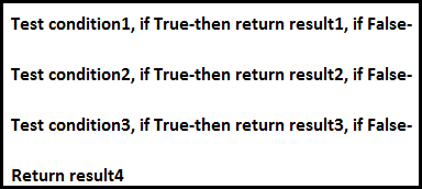
IF (condition1, result1, IF (condition2, result2, IF (condition3, result3,………..)))
Examples
You can download this Multiple Ifs Excel Template here – Multiple Ifs Excel Template
Example #1
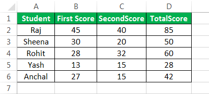
Suppose we wish to find how a student scores in an exam. There are two exam scores of a student, and we define the total score (sum of the two scores) as “Good,” “Average,” and “Bad.” A score would be “Good” if it is greater than or equal to 60, ‘Average’ if it is between 40 and 60, and ‘Bad’ if it is less than or equal to 40.
Let us say the first score is stored in column B, the second in column C.
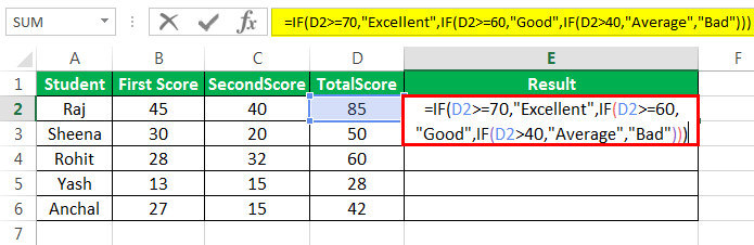
The following formula tells Excel to return “Good,” “Average,” or “Bad”:
=IF(D2>=60,”Good”,IF(D2>40,”Average”,”Bad”))
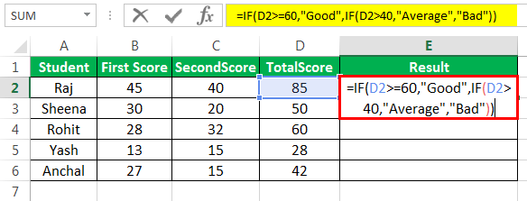
This formula returns the result as given below:
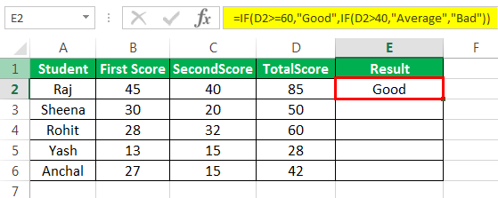
Drag the formula to get results for the rest of the cells.
We can see that one multiple IF function is sufficient in this case as we need to get only 3 results.
We can see that one multiple IF function is sufficient in this case as we need to get only 3 results.
Example #2
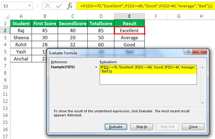
We want to test one more condition in the above examples: the total score of 70 and above is categorized as “Excellent.”
=IF(D2>=70,”Excellent”,IF(D2>=60,”Good”,IF(D2>40,”Average”,”Bad”)))
This formula returns the result as given below:
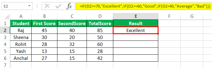
Excellent: >=70
Good: Between 60 & 69
Average: Between 41 & 59
Bad: <=40
Drag the formula to get results for the rest of the cells.
We can add several “IF” conditions if required similarly.
Example #3
Suppose we wish to test a few sets of different conditions. In that case, those conditions can be expressed using logical OR and AND, nesting the functions inside IF statements and then nesting the IF statements into each other.
For instance, if we have two columns containing the number of targets made by an employee in 2 quarters: Q1 and Q2. Then, we wish to calculate the performance bonus of the employee based on a higher target number.
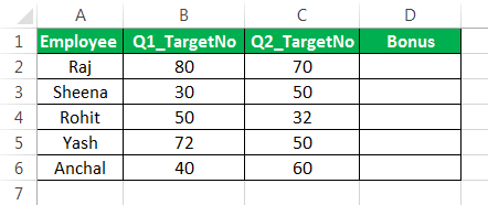
We can make a formula with the logic:
- If either Q1 or Q2 targets are greater than 70, then the employee gets a 10% bonus,
- If either of them is greater than 60, then the employee receives a 7% bonus,
- If either of them is greater than 50, then the employee gets a 5% bonus,
- If either is greater than 40, then the employee receives a 3% bonus. Else, no bonus.
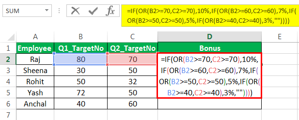
So, we first write a few OR statements like (B2>=70,C2>=70), and then nest them into logical tests of IF functions as follows:
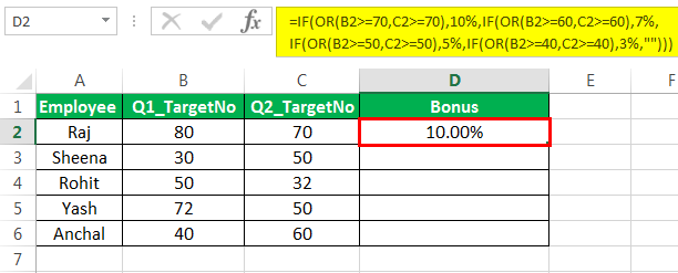
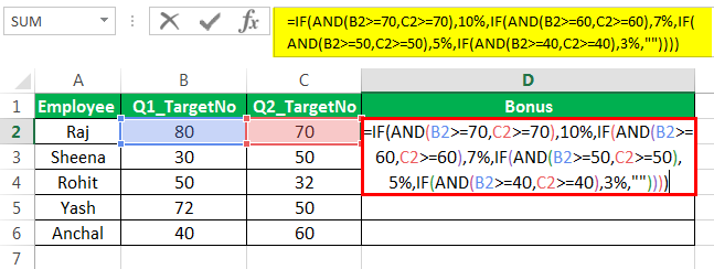
=IF(OR(B2>=70,C2>=70),10%,IF(OR(B2>=60,C2>=60),7%, IF(OR(B2>=50,C2>=50),5%, IF(OR(B2>=40,C2>=40),3%,””))))
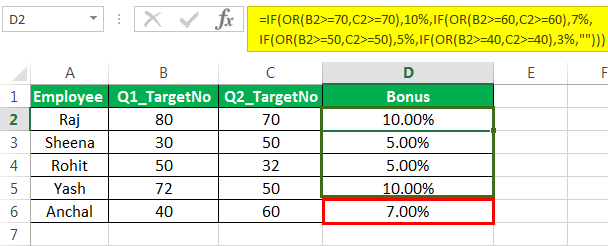
This formula returns the result as given below:
Next, drag the formula to get the results of the rest of the cells.
Example #4
Now, let us say we want to test one more condition in the above example:
- If both Q1 and Q2 targets are greater than 70, then the employee gets a 10% bonus
- if both of them are greater than 60, then the employee receives a 7% bonus
- if both of them are greater than 50, then the employee gets a 5% bonus
- if both of them are greater than 40, then the employee receives a 3% bonus
- Else, no bonus.
So, we first write a few AND statements like (B2>=70,C2>=70), and then nest them: tests of IF functions as follows:
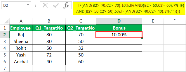
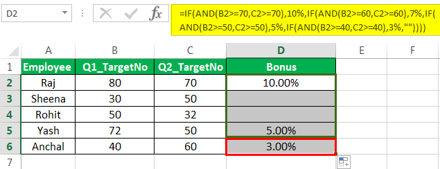
=IF(AND(B2>=70,C2>=70),10%,IF(AND(B2>=60,C2>=60),7%, IF(AND(B2>=50,C2>=50),5%, IF(AND(B2>=40,C2>=40),3%,””))))
This formula returns the result as given below:
Next, drag the formula to get results for the rest of the cells.
Things to Remember
- The multiple IF function evaluates the logical tests in the order they appear in a formula. So, for example, as soon as one condition evaluates to be “True,” the following conditions are not tested.
- For instance, if we consider the second example discussed above, the multiple IF condition in Excel evaluates the first logical test (D2>=70) and returns “Excellent” because the condition is “True” in the below formula:
=IF(D2>=70,”Excellent”,IF(D2>=60,,”Good”,IF(D2>40,”Average”,”Bad”))
Now, if we reverse the order of IF functions in Excel as follows:
=IF(D2>40,”Average”,IF(D2>=60,,”Good”,IF(D2>=70,”Excellent”,”Bad”))
In this case, the formula tests the first condition. Since 85 is greater than or equal to 70, a result of this condition is also “True,” so the formula would return “Average” instead of “Excellent” without testing the following conditions.
Correct Order

Incorrect Order
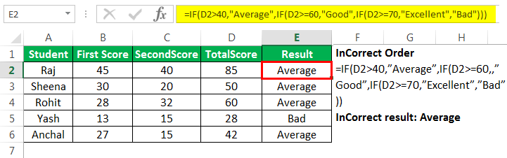
Note: Changing the order of the IF function in Excel would change the result.
- Evaluate the formula logic– To see the step-by-step evaluation of multiple IF conditions, we can use the ‘Evaluate Formula’ feature in excel on the “Formula” tab in the “Formula Auditing” group. Clicking the “Evaluate” button will show all the steps in the evaluation process.
- For instance, in the second example, the evaluation of the first logical testA logical test in Excel results in an analytical output, either true or false. The equals to operator, “=,” is the most commonly used logical test.read more of multiple IF formulas will go as D2>=70; 85>=70; True; Excellent.
- Balancing the parentheses: If the parentheses do not match in terms of number and order, then the multiple IF formula would not work.
- If we have more than one set of parentheses, the parentheses pairs are shaded in different colors so that the opening parentheses match the closing ones.
- Also, on closing the parenthesis, the matching pair is highlighted.
- Numbers and Text should be treated differently: The text should always be enclosed in double quotes in the multiple IF formula.
- Multiple IF’s can often become troublesome: Managing many true and false conditions and closing brackets in one statement becomes difficult. Therefore, it is always good to use other tools like IF function or VLOOKUP in case Multiple IF’sSometimes while working with data, when we match the data to the reference Vlookup, it finds the first value and does not look for the next value. However, for a second result, to use Vlookup with multiple criteria, we need to use other functions with it.read more are difficult to maintain in Excel.
Recommended Articles
This article is a guide to Multiple IF Conditions in Excel. We discuss using multiple IF conditions, practical examples, and a downloadable Excel template. You may also learn more about Excel from the following articles: –
- IF OR in VBAIF OR is not a single statement; it is a pair of logical functions used together in VBA when we have more than one criteria to check, and when we use the if statement, we receive the true result if either of the criteria is met.read more
- COUNTIF in ExcelThe COUNTIF function in Excel counts the number of cells within a range based on pre-defined criteria. It is used to count cells that include dates, numbers, or text. For example, COUNTIF(A1:A10,”Trump”) will count the number of cells within the range A1:A10 that contain the text “Trump”
read more - IFERROR Excel Function – ExamplesThe IFERROR function in Excel checks a formula (or a cell) for errors and returns a specified value in place of the error.read more
- SUMIF Excel FunctionThe SUMIF Excel function calculates the sum of a range of cells based on given criteria. The criteria can include dates, numbers, and text. For example, the formula “=SUMIF(B1:B5, “<=12”)” adds the values in the cell range B1:B5, which are less than or equal to 12.
read more
We use the IF statement in Excel to test one condition and return one value if the condition is met and another if the condition is not met.
However, we use multiple or nested IF statements when evaluating numerous conditions in a specific order to return different results.
This tutorial shows four examples of using nested IF statements in Excel and gives five alternatives to using multiple IF statements in Excel.
General Syntax of Nested IF Statements (Multiple IF Statements)
The general syntax for nested IF statements is as follows:
=IF(Condition1, Value_if_true1, IF(Condition2, Value_if_true2, IF(Condition3, Value_if_true3, Value_if_false)))
This formula tests the first condition; if true, it returns the first value.
If the first condition is false, the formula moves to the second condition and returns the second value if it’s true.
Each subsequent IF function is incorporated into the value_if_false argument of the previous IF function.
This process continues until all conditions have been evaluated, and the formula returns the final value if none of the conditions is true.
The maximum number of nested IF statements allowed in Excel is 64.
Now, look at the following four examples of how to use nested IF statements in Excel.
Example #1: Use Multiple IF Statements to Assign Letter Grades Based on Numeric Scores
Let’s consider the following dataset showing some students’ scores on a Math test.

We want to use nested IF statements to assign student letter grades based on their scores.
We use the following steps:
- Select cell C2 and type in the below formula:
=IF(B2>=90,"A",IF(B2>=80,"B",IF(B2>=70,"C",IF(B2>=60,"D","F"))))

- Click Enter in the cell to get the result of the formula in the cell.
- Copy the formula for the rest of the cells in the column
The assigned letter grades appear in column C.

Explanation of the formula
=IF(B2>=90,”A”,IF(B2>=80,”B”,IF(B2>=70,”C”,IF(B2>=60,”D”,”F”))))
This formula evaluates the value in cell B2 and assigns an “A” if the value is 90 or greater, a “B” if the value is between 80 and 89, a “C” if the value is between 70 and 79, a “D” if the value is between 60 and 69, and an “F” if the value is less than 60.
Notice that it can be challenging to keep track of which parentheses go with which arguments in nested IF functions.
Therefore, as we enter the formula, Excel uses different colors for the parentheses at each level of the nested IF functions to make it easier to see which parts of the formula belong together.

Also read: How to use Excel If Statement with Multiple Conditions Range
Example #2: Use Multiple IF Statements to Calculate Commission Based on Sales Volume
Here’s the dataset showing the sales of specific salespeople in a particular month.

We want to use multiple IF statements to calculate the tiered commission for the salespeople based on their sales volume.
We proceed as follows:
- Select cell C2 and enter the following formula:
=IF(B2>=40000, B2*0.14,IF(B2>=20000,B2*0.12,IF(B2>=10000,B2*0.105,IF(B2>0,B2*0.08,0))))

- Press the Enter key to get the result of the formula.
- Double-click or drag the Fill Handle to copy the formula down the column.
The commission for each salesperson is displayed in column D.

Explanation of the formula
=IF(B2>=40000, B2*0.14,IF(B2>=20000,B2*0.12,IF(B2>=10000,B2*0.105,IF(B2>0,B2*0.08,0))))
This formula evaluates the value in cell B2 and then does the following:
- If the value in cell B2 is greater than or equal to 40,000, the figure is multiplied by 14% (0.14).
- If the figure in cell B2 is less than 40,000 but greater than or equal to 20,000, the value is multiplied by 12% (0.12).
- If the number in cell B2 is less than 20,000 but greater than or equal to 10,000, the figure is multiplied by 10.5% (0.105).
- If the value in cell B2 is less than 10,000 but greater than 0 (zero), the number is multiplied by 8% (0.08).
- If the value in cell B2 is 0 (zero), 0 (zero) is returned.
Example #3: Use Multiple IF Statements to Assign Sales Performance Rating Based On Sales Target Achievement
The following is a dataset showing regional sales data of a specific technology company in a particular year.

We want to use multiple IF statements to assign a sales performance rating to each region based on their sales target achievement.
We use the following steps:
- Select cell C2 and type in the below formula:
=IF(B2>500000, "Excellent", IF(B2>400000, "Good", IF(B2>275000, "Average", "Poor")))

- Click Enter on the Formula bar.
- Drag or double-click the Fill Handle to copy the formula down the column.
The performance ratings of the regions are shown in column C.

Explanation of the formula
=IF(B2>500000, “Excellent”, IF(B2>400000, “Good”, IF(B2>275000, “Average”, “Poor”)))
In this formula, if the sales target in cell B2 is greater than 500,000, the formula returns “Excellent.”
If it’s between 400,000 and 500,000, the formula returns “Good.”
If it’s between 275,000 and 400,000, the formula returns “Average.” And if it’s below 275,000, the formula returns “Poor.”
Example #4: Use Multiple IF Statements in Excel to Check For Errors and Return Error Messages
Suppose we have the following dataset of students’ English test scores. Some scores are less than 0 or greater than 100, and there are no scores in some cases.

We want to use nested IF statements to check for scores in column B and display error messages in column C if there are no scores or the scores are less than 0 or greater than 100.
If the score in column B is valid, we want the formula to return an empty string in column C.
Here are the steps to follow:
- Select cell C2 and enter the following formula:
=IF(OR(B2<0,B2>100),"Score out of range",IF(ISBLANK(B2),"Invalid score",""))

- Click Enter on the Formula bar.
- Drag the Fill Handle to copy the formula down the column.
The error messages are shown in column C.

Explanation of the formula
=IF(OR(B2<0,B2>100),”Score out of range”,IF(ISBLANK(B2),”Invalid score”,””))
This formula uses the OR function to check if the score in cell B2 is less than 0 or greater than 100, and if it is, it returns the error message “Score out of range.”
The formula also uses the ISBLANK function to check if cell B2 is blank, and if it is, it returns the error message “Invalid score.”
If there is no error, the formula returns an empty string, meaning no message is displayed in column B.
Alternatives to Using Multiple IF Statements in Excel
Formulas using nested IF statements can become difficult to read and manage if we have more than a few conditions to test.
In addition, if we exceed the maximum allowed limit of 64 nested IF statements, we will get an error message.
Fortunately, Excel offers alternative ways to use instead of nested IF functions, especially when we need to test more than a few conditions.
We present the alternative ways in this tutorial.
Alternative #1: Use the IFS Function
The IFS function tests whether one or more conditions are met and returns a value corresponding to the first TRUE condition.
Before the release of the IFS function in 2018 as part of the Excel 365 update, the only way to test multiple conditions and return a corresponding value in Excel was to use nested IF statements.
However, multiple IF statements have the downside of resulting in unwieldy formulas that are difficult to read and maintain.
In some situations, the IFS function is designed to replace the need for multiple IF functions.
The syntax of the IFS function is more straightforward and easier to read than nested IF statements, and it can handle up to 127 conditions.
Here’s an example:
Let’s consider the following dataset showing some students’ scores on a Math test.

We want to use the IFS function to assign letter grades to the students based on their scores.
We use the following steps:
- Select cell C2 and type in the below formula:
=IFS(B2>=90, "A", B2>=80, "B", B2>=70, "C", B2>=60, "D", B2<60, "F")

- Click Enter on the Formula bar.
- Drag or double-click the Fill Handle to copy the formula down the column.
The student’s letter grades are shown in column C.

Explanation of the formula
=IFS(B2>=90, “A”, B2>=80, “B”, B2>=70, “C”, B2>=60, “D”, B2<60, “F”)
This formula tests the score in cell B2 against each condition and returns the corresponding grade letter when the condition is true.
Limitation of IFS Function
The IFS function in Excel is designed to simplify complex nested IF statements.
However, there are situations where the IFS function may not be able to replace nested IF functions completely.
One such situation is when you must calculate or operate based on a condition or set of conditions.
While the IFS function can return a value or text string based on a condition, it cannot perform calculations or operations on that value like nested IF statements.
Another situation where the IFS function may be less useful is when you need to test for a range of conditions rather than just a specific set.
This is because the IFS function requires you to specify each condition and corresponding result separately, which can become cumbersome if you have many conditions to test—in contrast, nested IF statements allow you to test for a range of conditions using logical operators like AND and OR.
The IFS function is a powerful tool for simplifying complex logical tests in Excel.
However, there may be situations where nested IF statements are more appropriate for your needs.
We recommend that you consider both options and choose the one that best fits the specific requirements of your task.
Alternative #2: Use Nested IF Functions
We can use multiple IFS functions in a formula if we have more than one condition to test.
For example, let’s say we have the following dataset of student names and scores on a Physics test in columns A and B.

We want to assign a letter grade to each score and include a pass or fail designation based on whether the score is above or below 75.
Here are the steps to use:
- Select cell C2 and enter the following formula
=IFS(B2>=90,"A",B2>=80,"B",B2>=70,"C",B2>=60,"D",B2<60,"F")&" "&IFS(B2>=75,"Pass",B2<75,"Fail")

- Click Enter on the Formula bar.
- Drag or double-click the Fill Handle to copy the formula down the column.
The letter grade and designation of the student scores are displayed in column C.

Explanation of the formula
=IFS(B2>=90,”A”,B2>=80,”B”,B2>=70,”C”,B2>=60,”D”,B2<60,”F”)&” “&IFS(B2>=75,”Pass”,B2<75,”Fail”)
This formula uses the first IFS function to assign a letter grade based on the score in column A and the second IFS function to give a pass/fail designation based on the score in column A.
The two IFS functions are combined using the ampersand (&) operator to create a single text string that displays each score’s letter grade and pass/fail designation.
Alternative #3: Use the Combination of CHOOSE and XMATCH Functions
The CHOOSE function selects a value or action from a value list based on an index number.
The XMATCH function locates and returns the relative position of an item in an array. We can combine these functions in a formula instead of nested IF functions.
Here’s an example:
Suppose we have the following dataset showing some students’ scores and letter grades on a Biology test.

We want to use a formula combining the CHOOSE and XMATCH functions to assign corresponding grade points in column D to each letter grade.
We use the following steps:
- Select cell D2 and type in the below formula:
=CHOOSE(XMATCH(C2,{"F","E","D","C","B","A"},0),0,1,2,3,4,5)

- Click Enter on the Formula bar.
- Drag or double-click the Fill Handle to copy the formula down the column.
The grade points for each student are displayed in column D.

Explanation of the formula
=CHOOSE(XMATCH(C2,{“F”,”E”,”D”,”C”,”B”,”A”},0),0,1,2,3,4,5)
This formula applies the XMATCH function to find the position of the letter grade in the array {“F”,”E”,”D”,”C”,”B”,”A”}, and then uses the CHOOSE function to return the corresponding grade points.
Alternative #4: Use the VLOOKUP Function
The VLOOKUP function looks for a value in the leftmost column of a table and then returns a value in the same row from a specified column.
We can use the VLOOKUP function instead of nested IF functions in Excel.
The following is an example of using the VLOOKUP function instead of nested IF functions in Excel:
Suppose we have the following dataset showing some students’ scores and letter grades on a Biology test.

We want to use the VLOOKUP function to assign grade points to each student’s letter grade in column D.
We use the steps below:
- Create a table that lists the grades and their corresponding grade points in cell range F1:G7.

- In cell D2, type the following formula:
=VLOOKUP(C2,$F$2:$G$7,2,FALSE)
Note: Use the dollar signs to lock down the cell range F2:G7.

- Click Enter on the Formula bar.
- Drag or double-click the Fill Handle to copy the formula down the column.
The grade points for each student appear in column D.

Explanation of the formula
=VLOOKUP(C2,$F$2:$G$7,2,FALSE)
This formula uses the VLOOKUP function to look up the grade in cell C2 in the table in F2:G7 and return the corresponding grade point in the second column (i.e., column G).
The “FALSE” argument ensures that an exact match is required.
Alternative #5: Use a User-Defined Function
If you need to test more than a few conditions, consider creating a User Defined Function in VBA that can handle many conditions.
Here’s an example of using VBA code to replace nested IF functions in Excel:
Suppose we have the following dataset showing the sales of specific salespeople in a particular month.

We want to use a User Defined Function to calculate the commission for each salesperson based on the following rates:
- If the total sales are less than $10,000, the commission rate is 8%.
- If the total sales are equal to or greater than $10,000 but less than $20,000, the commission rate is 10.5%.
- If the total sales are equal to or greater than $20,000 but less than $40,000, the commission rate is 12%.
- If the sales are equal to or greater than $40,000, the commission rate is 14%
We use the following steps:
- Open the worksheet containing the sales dataset.
- Press Alt + F11 to launch the Visual Basic Editor.
- Click Insert on the menu bar and choose Module to insert a new module.

- Enter the following VBA code.
'Code developed by Steve Scott from https://spreadsheetplanet.com
Function COMMISSION(Sales As Double) As Double
    Const Rate1 = 0.08
    Const Rate2 = 0.105
    Const Rate3 = 0.12
    Const Rate4 = 0.14

'Calculate sales commissions

    Select Case Sales
        Case 0 To 9999.99: COMMISSION = Sales * Rate1
        Case 10000 To 19999.99: COMMISSION = Sales * Rate2
        Case 20000 To 39999.99: COMMISSION = Sales * Rate3
        Case Is >= 40000: COMMISSION = Sales * Rate4
    End Select

End Function
- Save the function procedure and the workbook as a Macro-Enabled Workbook.
- Press Alt + F11 to switch to the active worksheet with the sales dataset.
- Select cell C2 and enter the following formula:
=COMMISSION(B2)

- Click Enter on the Formula bar.
- Drag or double-click the Fill Handle to copy the formula down the column.
The commission for each salesperson is displayed in column C.

This VBA function takes the sales amount as an argument and returns the corresponding commission.
The User-Defined Function is a much simpler and easier-to-read solution than using nested IF functions.
This tutorial showed four examples of using nested IF statements in Excel and gave five alternatives to using multiple IF statements in Excel. We hope you found the tutorial helpful.
Other Excel tutorials you may find useful:
- Excel Logical Test Using Multiple If Statements in Excel [AND/OR]
- How to Compare Two Columns in Excel (using VLOOKUP & IF)
- Using IF Function with Dates in Excel (Easy Examples)
- COUNTIF Greater Than Zero in Excel
- BETWEEN Formula in Excel (Using IF Function) – Examples
- Count Cells Less than a Value in Excel (COUNTIF Less)
Логическая функция ЕСЛИ в Экселе – одна из самых востребованных. Она возвращает результат (значение или другую формулу) в зависимости от условия.
Функция имеет следующий синтаксис.
ЕСЛИ(лог_выражение; значение_если_истина; [значение_если_ложь])
лог_выражение – это проверяемое условие. Например, A2<100. Если значение в ячейке A2 действительно меньше 100, то в памяти эксель формируется ответ ИСТИНА и функция возвращает то, что указано в следующем поле. Если это не так, в памяти формируется ответ ЛОЖЬ и возвращается значение из последнего поля.
значение_если_истина – значение или формула, которое возвращается при наступлении указанного в первом параметре события.
значение_если_ложь – это альтернативное значение или формула, которая возвращается при невыполнении условия. Данное поле не обязательно заполнять. В этом случае при наступлении альтернативного события функция вернет значение ЛОЖЬ.
Очень простой пример. Нужно проверить, превышают ли продажи отдельных товаров 30 шт. или нет. Если превышают, то формула должна вернуть «Ок», в противном случае – «Удалить». Ниже показан расчет с результатом.

Продажи первого товара равны 75, т.е. условие о том, что оно больше 30, выполняется. Следовательно, функция возвращает то, что указано в следующем поле – «Ок». Продажи второго товара менее 30, поэтому условие (>30) не выполняется и возвращается альтернативное значение, указанное в третьем поле. В этом вся суть функции ЕСЛИ. Протягивая расчет вниз, получаем результат по каждому товару.
Однако это был демонстрационный пример. Чаще формулу Эксель ЕСЛИ используют для более сложных проверок. Допустим, есть средненедельные продажи товаров и их остатки на текущий момент. Закупщику нужно сделать прогноз остатков через 2 недели. Для этого нужно от текущих запасов отнять удвоенные средненедельные продажи.

Пока все логично, но смущают минусы. Разве бывают отрицательные остатки? Нет, конечно. Запасы не могут быть ниже нуля. Чтобы прогноз был корректным, нужно отрицательные значения заменить нулями. Здесь отлично поможет формула ЕСЛИ. Она будет проверять полученное по прогнозу значение и если оно окажется меньше нуля, то принудительно выдаст ответ 0, в противном случае — результат расчета, т.е. некоторое положительное число. В общем, та же логика, только вместо значений используем формулу в качестве условия.

В прогнозе запасов больше нет отрицательных значений, что в целом очень неплохо.
Формулы Excel ЕСЛИ также активно используют в формулах массивов. Здесь мы не будем далеко углубляться. Заинтересованным рекомендую прочитать статью о том, как рассчитать максимальное и минимальное значение по условию. Правда, расчет в той статье более не актуален, т.к. в Excel 2016 появились функции МИНЕСЛИ и МАКСЕСЛИ. Но для примера очень полезно ознакомиться – пригодится в другой ситуации.
Формула ЕСЛИ в Excel – примеры нескольких условий
Довольно часто количество возможных условий не 2 (проверяемое и альтернативное), а 3, 4 и более. В этом случае также можно использовать функцию ЕСЛИ, но теперь ее придется вкладывать друг в друга, указывая все условия по очереди. Рассмотрим следующий пример.
Нескольким менеджерам по продажам нужно начислить премию в зависимости от выполнения плана продаж. Система мотивации следующая. Если план выполнен менее, чем на 90%, то премия не полагается, если от 90% до 95% — премия 10%, от 95% до 100% — премия 20% и если план перевыполнен, то 30%. Как видно здесь 4 варианта. Чтобы их указать в одной формуле потребуется следующая логическая структура. Если выполняется первое условие, то наступает первый вариант, в противном случае, если выполняется второе условие, то наступает второй вариант, в противном случае если… и т.д. Количество условий может быть довольно большим. В конце формулы указывается последний альтернативный вариант, для которого не выполняется ни одно из перечисленных ранее условий (как третье поле в обычной формуле ЕСЛИ). В итоге формула имеет следующий вид.

Комбинация функций ЕСЛИ работает так, что при выполнении какого-либо указанно условия следующие уже не проверяются. Поэтому важно их указать в правильной последовательности. Если бы мы начали проверку с B2<1, то условия B2<0,9 и B2<0,95 Excel бы просто «не заметил», т.к. они входят в интервал B2<1 который проверился бы первым (если значение менее 0,9, само собой, оно также меньше и 1). И тогда у нас получилось бы только два возможных варианта: менее 1 и альтернативное, т.е. 1 и более.
При написании формулы легко запутаться, поэтому рекомендуется смотреть на всплывающую подсказку.

В конце нужно обязательно закрыть все скобки, иначе эксель выдаст ошибку

Функция Excel ЕСЛИМН
Функция Эксель ЕСЛИ в целом хорошо справляется со своими задачами. Но вариант, когда нужно записывать длинную цепочку условий не очень приятный, т.к., во-первых, написать с первого раза не всегда получается (то условие укажешь неверно, то скобку не закроешь); во-вторых, разобраться при необходимости в такой формуле может быть непросто, особенно, когда условий много, а сами расчеты сложные.
В MS Excel 2016 появилась функция ЕСЛИМН, ради которой и написана вся эта статья. Это та же ЕСЛИ, только заточенная специально для проверки множества условий. Теперь не нужно сто раз писать ЕСЛИ и считать открытые скобки. Достаточно перечислить условия и в конце закрыть одну скобку.
Работает следующим образом. Возьмем пример выше и воспользуемся новой формулой Excel ЕСЛИМН.

Как видно, запись формулы выглядит гораздо проще и понятнее.
Стоит обратить внимание на следующее. Условия по-прежнему перечисляем в правильном порядке, чтобы не произошло ненужного перекрытия диапазонов. Последнее альтернативное условие, в отличие от обычной ЕСЛИ, также должно быть обязательно указано. В ЕСЛИ задается только альтернативное значение, которое наступает, если не выполняется ни одно из перечисленных условий. Здесь же нужно указать само условие, которое в нашем случае было бы B2>=1. Однако этого можно избежать, если в поле с условием написать ИСТИНА, указывая тем самым, что, если не выполняются ранее перечисленные условия, наступает ИСТИНА и возвращается последнее альтернативное значение.
Теперь вы знаете, как пользоваться функцией ЕСЛИ в Excel, а также ее более современным вариантом для множества условий ЕСЛИМН.
Поделиться в социальных сетях:
The IF function is one of the most commonly used in Excel. The function can test a single condition as well as perform multiple complex logic tests. We can thus control the execution of Excel tasks using the IF function.
This is important since it enables us to perform actions depending on whether they meet certain conditions defined by the IF formula. We can also add data to cells using the function if other cells meet any of the conditions defined in the IF formula.
To add multiple conditions to an IF formula, we simply add nested IF functions.
In this article, you will learn the basics of the IF function and how to come up with an array of IF formulas. You will also learn the nested IF’s function.
Let’s get started!
1. Basic IF formula that tests a single condition
A single IF statement tests whether a condition is met and returns a value if TRUE and another value if FALSE.
IF (logical test, ‘value_if_true’, ‘value_if_false’)
In the example below, let us test whether the price is less than or equal to 2000. If the condition is true return cheap, otherwise return expensive!
Go to Cell C2 and type ‘=IF(B2<=2000,»CHEAP», «EXPENSIVE»)’

The if formula above records or posts the String Good whenever the single condition B2<=2000.
2. IF formula with multiple conditions (Nested IF Functions.
If you have complex data or want to perform powerful data analysis, you might need to test multiple conditions at a time. You might need to perform a logical test across multiple conditions.
In such cases, you have to use an IF statement with multiple conditions/ranges in a single formula. These multiple IF conditions are normally called nested IF Functions. The function is used if want more than 3 different results.
The general syntax for IF function with multiple conditions is
=IF (condition one is true, do something, IF (condition two is true, do something, IF (conditions three is true, do something, else do something)))
Commas are used to separate conditions and IF functions in the IF formula. The «)» is used to close all IFs at the End of the formula while the » (» opens all IF functions. The number of «(» should be equal to that of «)».
In our above example, we can include multiple conditions in the IF formula as follows
=IF(B2<=2000,»CHEAP»,IF(B2<=6000,»AFFORDABLE»,IF(B2<=10000,»EXPENSIVE»,»LUXURIOUS»)))

Press Enter to get the results and use the AutoFill feature to copy the formula to the rest of the cells.

3. IF formula with logical test
You can use an IF statement with AND and OR conditions to perform a logical test. IF your formula has AND function, the logical test returns TRUE if all the conditions are met; otherwise, it will return FALSE. While the OR Function returns TRUE if any of the conditions is met; otherwise it returns FALSE.
3.1 IF with AND Function
In the example below, a student is deemed to pass the exam if he/she has a score of 42 in Maths and 50 in English.

With this information, we can write the condition as follows;
AND (C14>=42, D14>=50)
To know whether the student passed or failed the exam. You can use the IF statement.
= IF(AND (C14>=42, D14>=50),”PASS”,”FAIL”)

Press enter and use the AutoFill feature to copy the formula to the rest of the cells.

3.2 IF with OR Function
The IF with OR Function works the same way as the AND function we have seen above. The only difference is that, if one of the conditions is TRUE then the result will be TRUE.
Follow the above process to apply the OR Function.
In cell E14, type = IF(OR (C14>=42, D14>=50),”PASS”,”FAIL”)

Press enter to get the results.

3. IF with ISNUMBER and ISTEXT Functions
You can use ISNUMBER and ISTEXT formula to find whether the cells have text value, number, or blank.
=IF(ISTEXT(A1), «Text», IF(ISNUMBER(A1), «Number», IF(ISBLANK(A1), «Blank», «»)))

You can only apply AND & OR functions at a time if your task requires you to evaluate several sets of conditions. For example, if you are checking exam results using these criteria:
Condition 1: exam1>50 and exam2>50
Condition 2: exam1>40 and exam2>60
In this case, the exam is deemed passed if either of the conditions is passed.
Although the formula may seem tricky, you only need to express each condition as an AND statement and nest them in the OR function. That is because meeting all the conditions is not necessary, but either statement will serve the purpose. Therefore, the general formula will be:
OR(AND(B2>50, C2>50), AND(B2>40, C2>60)
You can now use the OR function to test the logic of IF and supply the desired value_if_true and value_if_false values. In the end, the final IF formula with multiple AND & OR statements will turn into:
=IF(OR(AND(B2>50, C2>50), AND(B2>40, C2>60), «Pass», «Fail»)


5. Using the Array Formula
An Array formula can also help to get an Excel IF to test multiple conditions. For example, to evaluate the AND logical condition, you can use the asterisk:
IF(condition1) * (condition2) * …, value_if_true, value_if_false)
While to test conditions using OR logic, you will apply the plus sign:
IF(condition1) + (condition2) + …, value_if_true, value_if_false)
Finally, you can complete the Array formula by pressing Ctrl + Shift + Enter buttons together. The trick can also work as a regular formula in Excel 365 and Excel 2021 since it supports dynamic arrays.
Example: We can get “Pass” if cells B2 and C2 are greater than 50 by applying the formulas;
=IF((B2>50) * (C2>50), «Pass», «Fail») for AND logic


…, and
=IF((B2>50) + (C2>50), «Pass», «Fail») for OR logic.


6. IF With Other Excel Functions
Other Excel functions that can give the IF formula for multiple conditions include
6.1 IF#N/A Error in VLOOKUP Function
The VLOOKUP or any other lookup function returns a N/A error if it cannot find something. Therefore, you can return zero, blank, or text if #N/A to make your table neat. Here, you will need the following generic formula:
IF(ISNA(VLOOKUP(…)), value_if_na, VLOOKUP(…))
Example 1. If the lookup value in a cell (E1) is not found, the formula returns 0 as shown below;
=IF(ISNA(VLOOKUP(E1, A2:B10, 2,FALSE )), 0, VLOOKUP(E1, A2:B10, 2, FALSE))

Example 2: If the lookup value is not found, the formula returns blank as shown below;
=IF(ISNA(VLOOKUP(E1, A2:B10, 2,FALSE )), «», VLOOKUP(E1, A2:B10, 2, FALSE))

Example 3: If the lookup value is not available, the formula returns a specific text as shown below;
=IF(ISNA(VLOOKUP(E1, A2:B10, 2,FALSE )), «Not found», VLOOKUP(E1, A2:B10, 2, FALSE))

6.2 IF With SUM, AVERAGE, MIN, and MAX Functions
Excel has the SUMIF and SUMIFS functions that you can use, to sum up values in cells using certain criteria. You can use the SUM function to test the IF logic of your business. For instance, you can apply this formula to determine the text labels based on the sum of cells B2 and C2 values;
=IF(SUM(B2:C2)>130, «Good», IF(SUM(B2:C2)>110, «Satisfactory», «Poor»))

From the formula, the return text label is “Good” if the sum of the two cells is greater than 130. If the sum is greater than 110, the return text is “Satisfactory”, while if the sum is 110 or below, the return text is “Poor”.
You can still embed the AVERAGE function similarly to test the IF logic and return a different text label based on the average score of the two cells. In this case, the generic formula will be;
=IF(AVERAGE(B2:C2)>65, «Good», IF(AVERAGE(B2:C2)>55, «Satisfactory», «Poor»))

If the sum of cells B2 and C2 is indicated in cell D2, you can use the MAX and MIN functions to identify the highest and lowest values through the formulas;
=IF(D2=MAX($D$2: $D$10), «Best result», «»)

=IF(D2=MAX($D$2: $D$10), «Best result», «»)

Lastly, you can nest the two functions into one another to have both text labels in one column to get the formula;
=IF(D2=MAX($D$2:$D$10), «Best result», IF(D2=MIN($D$2:$D$10), «Worst result», «»))

6.3 IF with CONCATENATE Function
You can also use the CONCATENATE and IF functions to output the result of IF and some text into one cell. Here, you can use the formula;
=CONCATENATE(«You performed «, IF(B1>100,»fantastic!», IF(B1>50, «well», «poor»)))

From the formula, the student will get a «fantastic» result if the score in cell B1 is greater than 100. On the other hand, the result will be «well» if the score in cell B1 is greater than 50.
6.4 IF with ISERROR and ISNA Functions
These functions can only work in modern Excel versions where they trap and replace errors with another predefined value. For instance, the IFERROR function works in Excel 2007 and later, while the IFNA function works in Excel 2013 and later. When using earlier Excel versions, you will need the combinations of IF ISERROR and IF ISNA. So, what is the difference between these applications?
The answer is simple: IFERROR and ISERROR functions can handle all the possible errors resulting from Excel calculations, including VALUE, N/A, NAME, REF, NUM, DIV/0, and NULL errors. Contrary, IFNA, and ISNA handle only N/A errors.
Example: If you want to replace the #DIV/0 (divide by zero error) with a predefined text or value, you can use the formula;
=IF(ISERROR(A2/B2), «N/A», A2/B2), where;
A2 represents the value in cell A2
B2 represents the value in cell B2.
A2/B2 represents the results attained after dividing A2 by B2.
If the value in cell B2 is 0, the formula will return a N/A text.

I hope you found this tutorial useful.

What is Multiple IF Statements?
Multiple IF statements are also known as “Nested IF Statement” is a formula containing 2 or more IF functions. A single IF function only analyze two criteria. If there are more than two criteria, then it should use the multiple IF statements (nested IF). The number of IF functions required in multiple IF statements is the number of criteria minus 1.
Multiple IF Statements in Excel
What is the weight category of each name below based on BMI value? to get the value of BMI, divide the weight (in KG) by the height (in Meter2)

The following is a weight category based on BMI value.

There are six criteria means it takes 5 IF function to assemble multiple IF statements.
IF Function #1 – Underweight or Not
The first IF function looking for “Who has Underweight Body and Who is Not.”
Here are the steps to write the first IF function.
- Place the cursor in cell E2
- Type the formula for the IF Function
- logical_test argument, analyze whether the BMI value is less than 18.5?, type D2<18.5
- value_if_true argument, type “Underweight”
- value_if_false argument, type “” (blank space)
Look below for the resulting formula
=IF(D2<18.5,"Underweight","")
Do a copy in cell E2, then do a paste in range E3:13. The results are as shown below.

The result is two names in “Underweight” category; the other ten names are not in the underweight category. There are five possibilities; it could be Normal, Overweight, Class I Obesity, Class II Obesity or Class III Obesity.
Who has the ideal body? Second IF function answer the question.
IF Function #2 – Normal Weight or Not
The second IF function fills the value_if_false argument of the first IF function. The second IF function is searching “Who has Normal Weight Body and Who is Not.”
Here are the steps to write the second IF function.
- Edit the formula in cell E2 by pressing F2 key
- Change value_if_false argument of first IF function from “” to the second IF function
- logical_test argument, analyze whether the BMI value is less than 25, D2<25
- value_if_true argument, type “Normal”
- value_if_false argument, type “” (blank space)
Look below for the resulting formula
=IF(D2<18.5,"Underweight"
,IF(D2<25,"Normal",""))
Do a copy in cell E2, then do a paste in range E3:13. The results are as shown below.

Two names in “Normal Weight” category and there are already four names and their weight category.
There are eight other names with no weight category. There are four possibilities; it could be Overweight, Class I Obesity, Class II Obesity or Class III Obesity.
Who has the overweight body? Third IF function answer the question.
IF Function #3 – Overweight or Not
The third IF function takes the value_if_false argument of the second IF function, seeking “Who has Overweight Body and Who is Not.”
Here are the steps to write the third IF function.
- Edit the formula in cell E2 by pressing F2 key
- Change value_if_false argument of second IF function from “” to the third IF function
- logical_test argument, analyze whether the BMI value is less than 30, D2<30
- value_if_true argument, type “Overweight”
- value_if_false argument, type “” (blank space)
Look below for the resulting formula
=IF(D2<18.5,"Underweight"
,IF(D2<25,"Normal"
,IF(D2<30,"Overweight","")))
Do a copy in cell E2, then do a paste in range E3:13. The results are as shown below.

Two additional names appear in “Overweight” category. There were six names known their weight category; there are still six other names not yet known. There are three possibilities left; it could be Class I Obesity, Class II Obesity or Class III Obesity.
Who has the class I obesity body? Fourth IF function answer the question.
IF Function #4 – Class I Obesity or Not
The fourth IF function occupies the value_if_false argument of the third IF function. The fourth IF function seeking “Who has a Class I Obesity Body and Who is Not.”
Here are the steps to write the fourth IF function.
- Edit the formula in cell E2 by pressing F2 key
- Change value_if_false argument of third IF function from “” to the fourth IF function
- logical_test argument, analyze whether the BMI value is less than 30, D2<35
- value_if_true argument, type “Class I Obesity”
- value_if_false argument, type “” (blank space)
Look below for the resulting formula
=IF(D2<18.5,"Underweight"
,IF(D2<25,"Normal"
,IF(D2<30,"Overweight"
,IF(D2<35,"Class I Obesity",""))))
Do a copy in cell E2, then do a paste in range E3:13. The results are as shown below.

Again, two additional names appear, but in “Class I Obesity” category. There were eight names known their weight category; there are four names remain unknown. There are remaining two possibilities; it could be Class II Obesity or Class III Obesity.
Who has the class II obesity body? Fifth IF function answer the question.
IF Function #5 – Class II Obesity or Class III Obesity
The fifth IF function, the last IF function to determine weight category for each name, it takes the value_if_false argument of the fourth IF function, looking for “Who has a Class II Obesity Body and Who is Not.”
Here are the steps to write the fifth IF function.
- Edit the formula in cell E2 by pressing F2 key
- Change value_if_false argument of fourth IF function from “” to the fifth IF function
- logical_test argument, analyze whether the BMI value is less than 30, D2<40
- value_if_true argument, type “Class II Obesity”
- value_if_false argument, type “” (blank space)
Look below for the resulting formula
=IF(D2<18.5,"Underweight"
,IF(D2<25,"Normal"
,IF(D2<30,"Overweight"
,IF(D2<35,"Class I Obesity"
,IF(D2<40,"Class II Obesity","")))))
Do a copy in cell E2, then do a paste in range E3:13. The results are as shown below.

There are still two names and unknown weight category, all if function already used. “Who has a Class III Obesity Body,” which if function answer this question?
If only one weight category left, then the last one takes the value_if_false argument of the fifth IF function.
Edit the formula in cell E2, change the value_if_false argument of fifth IF function from “” to “Class III Obesity.”
Look below for the resulting formula.
=IF(D2<18.5,"Underweight"
,IF(D2<25,"Normal"
,IF(D2<30,"Overweight"
,IF(D2<35,"Class I Obesity"
,IF(D2<40,"Class II Obesity","Class III Obesity")))))
Do a copy in cell E2, then do a paste in range E3:13. The results are as shown below.

Formula Challenge!!!
All IF functions above use the “<” operator. Is it possible to use “>”, “<=” or “> =” operator for multiple if statement above?
The result should not be different.
Video Tutorial for Multiple IF Statements
Here is a video explains step by step writing multiple IF statements one by one from the first IF function until the fifth IF function
The next video explains how to write all the IF functions at once
Another Alternative for Multiple IF Statements
IFS Function
The IFS function is available if you have an Office 365 subscription, make sure you have the latest version of Office 365. Microsoft provides the IFS function as an alternative and an improvement of nested IF, no need to use multiple IF statements to analyze more than two criteria.
With the same example above, what is the weight category of each name below based on BMI value? Here is a solution using the IFS function. Look below for the resulting formula.
=IFS(D2<18.5,"Underweight"
,D2<25,"Normal"
,D2<30,"Overweight"
,D2<35,"Class I Obesity"
,D2<40,"Class II Obesity"
,TRUE,"Class III Obesity")

It makes no difference, multiple IF statements result and IFS function result.
VLOOKUP Function
The VLOOKUP function instead of multiple IF statements? Yes, you are not wrong, you can use VLOOKUP function to analyze more than two criteria. The key is the TRUE value for the range_lookup argument.
Using the same example as the previous case, what is the weight category of each name below based on BMI value?. Here is a solution using the VLOOKUP function. Look below for the resulting formula.
=VLOOKUP(D12,$A$3:$C$8,3,TRUE)

What is the difference? The multiple IF statements vs. the VLOOKUP function result.
Which One is the Best to Analyze more than 2 Criteria
Multiple IF Statements vs. IFS Function vs. VLOOKUP Function, which one is your choice?
Multiple IF statements tend to be difficult to use for the inexperienced, especially more than 5 IF functions in a formula. The biggest weakness of nested IF is there is a maximum limit. Before Excel 2007, seven is the maximum number in one formula, after Excel 2007 you can use up to 64 IF functions in one formula.
Although the latest version of Excel can accommodate a lot of IF functions, multiple IF statements are not the best solution, try to avoid it as much as possible.
The IFS function is an improvement for multiple IF statements provided by Microsoft, able to analyze up to 127 criteria. The disadvantage appears if there are any additional criteria; all formula must be edited to accommodate the addition of new criteria.
What about the VLOOKUP function? What is the maximum number of criteria allowed to be analyzed? If there is a new criterion added, should the formula be edited?
There are no maximum criteria for the VLOOKUP function; the number of rows in the excel worksheet is the limitation.
Look at the VLOOKUP function above, a VLOOKUP function and a table answering all the questions. If there are new criteria, then add the criteria in the table, by using the dynamic named range, no need to change the formula at all.
For me VLOOKUP is my choice, what is yours?
Related Function
Function used in this article
Multiple IFS in Excel
The Multiple IFS function in Excel is a powerful and time-saving tool for checking multiple conditions in a single formula. It tests each condition in order and stops when it finds the true condition. Once it finds the true condition, it gives you the result that is associated with that condition.
What’s really great about this function is that it can check many conditions and give you a different value for each condition. This is different from the regular IF function, which can only check one condition and give you one of two results.
You can include up to 127 pairs of conditions and values in the Multiple IFS function. It’s compatible with Excel 2016 and later versions, including Excel for Microsoft 365.
Arguments
- Logical _test: This is a logical expression that can be either “TRUE” or “FALSE.”
- Value_if_true: This will return the value as TRUE if the specified condition is in sync.
- Value_if_false: This will return the value as FALSE if the specified condition is not met.
For example, the formula =IF(A2=2, “TRUE,” “FALSE”), checks if A2 is equal to 2. If it is, the formula will show “TRUE“. If A2 is not equal to 2, the formula will show “FALSE“.
In Excel, we can find the IF function categorized under the LOGICAL condition group in the FORMULAS menu, as shown in the screenshot below.
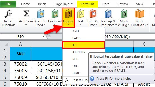
How to Use IF Function in excel?
Multiple IFS in Excel is very simple and easy. Let’s understand Multiple IFS in Excel, which are as below.
You can download this Multiple IFS Excel Template here – Multiple IFS Excel Template
Example #1 – Using IF Function in Excel
Consider the following table where students’ marks with the subject are shown:
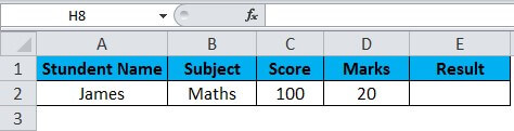
Here, we will use the IF condition to find out the student’s PASS or FAIL status by following the below steps.
- First, select cell E2. We want to display PASS or FAIL results in this cell.
- Enter the IF function – =IF(D2>C2, “PASS”, “FAIL”). Here, the IF function compares students’ marks in cell D2 with the passing marks in cell C2.
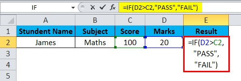
- Apply the formula and press enter to get the output as follows.
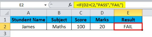
Result:
Since James’ marks (20) are less than the passing marks (100), the IF function returns the result as “FAIL“.
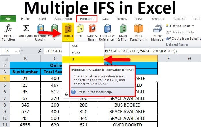
Example #2 – Multiple IFS in Excel with TEXT
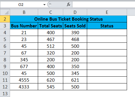
We will learn how to use the multiple IF function using a simple example. Consider the table below where we have an Online Bus Ticket Booking System, and we need to know the booking status of all the seats. We can derive the output using the Multiple IFS function in such cases.
To calculate the status for each booking using the IF function in Excel, follow these steps:
- Select the cell where it is necessary to display the status (in this case, E4).
- Type the equal sign (=) to begin the formula.
- Type the IF function and an opening bracket.
- Select the cell that contains the total seats (in this case, C4).
- Add the first condition: C4=D4 (total seats equal to sold).
- Type a comma.
- In double quotes, type “BUS BOOKED” to indicate a confirmed booking.
- Type another comma.
- Add the second condition: C4<D4 (total seats are less than seats sold).
- Type a comma.
- In double quotes, type “OVERBOOKED” to indicate more bookings than available seats.
- Type another comma.
- Then type “SPACE AVAILABLE” to show seats available for booking.
- Type the closing bracket for the IF function.
- Press Enter to apply the formula to the selected cell.
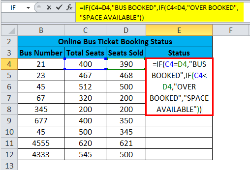
- Hence, the formula should look like this: =IF(C5=D5, “BUS BOOKED,” IF(C5<D5, “OVERBOOKED,” “SPACE AVAILABLE”))
- Once we apply the Multiple IFS, we will get the below output status:
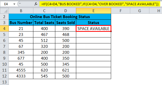
- In the example given, the IF function checks whether the value in cell A1 is less than 390. If the value exceeds or equals 390, the function returns the status as “OVERBOOKED” or “BUS BOOKED“, respectively. However, if the value is less than 390, the function returns “SPACE AVAILABLE” as the status. This function is useful for analyzing data and deciding based on specific conditions.
- Drag down the formula for all the cells so that we will get the below output result:
Result:
Example #3 – Multiple IFS Using Numeric Value
In this example, we will see how multiple IFS use numeric values to display the status.
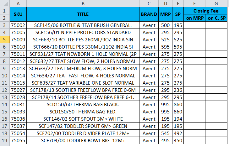
Consider the below example that shows MRP and SELLING PRICE, where we need to find out the closing FEE for Amazon titles. Here, we will use the Multiple IFS to get the CLOSING FEE for both the MRP AND SELLING PRICE by following the below steps:
- Here’s how we will apply the Multiple IF condition statement for MRP Closing Fee:
-
- Check if the MRP is less than $250. If it is, set the Closing Fee as Zero.
- The MRP is greater than or equal to $250, then check if it is less than 500 and if it is, set the closing fee as five (5).
- If the MRP is greater than or equal to 500, set the closing fee as ten (10).
-
- Here’s how we will apply the Multiple IF condition for the SELLING PRICE Closing Fee:
-
- Check if the Selling Price is less than $250 and if it is, the Closing Fee should be zero.
- If the Selling Price is between $250 and $499, the Closing Fee should be $5
- If the Selling Price is $500 or greater, the Closing Fee should be $10.
-
- We will apply the above two conditions by using the Multiple IFS in both columns.
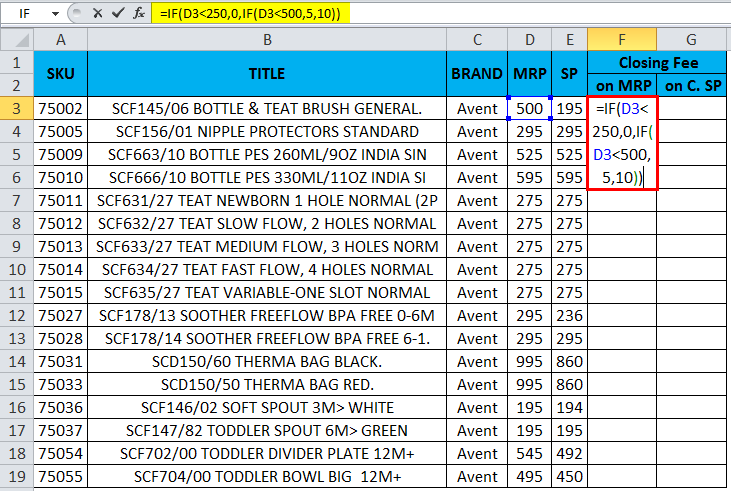
- First, insert the IF statement in F3.
- Begin by typing an opening bracket and selecting cell D3.
- Apply the condition: “D3<250” (indicating that the MRP is less than $250). Then, display the Closing Fee as zero and insert a comma.
- Next, insert another IF condition and open the brackets. Type the condition “D3<500” (indicating that the MRP is between $250 and $499).
- If this condition is met, display the Closing Fee as 5, and if not, display it as 10.
- Lastly, if we combine the above IF conditions, we will get the Multiple IFS statement shown as:
- Once we apply the Multiple IFS, we will get the below output status:
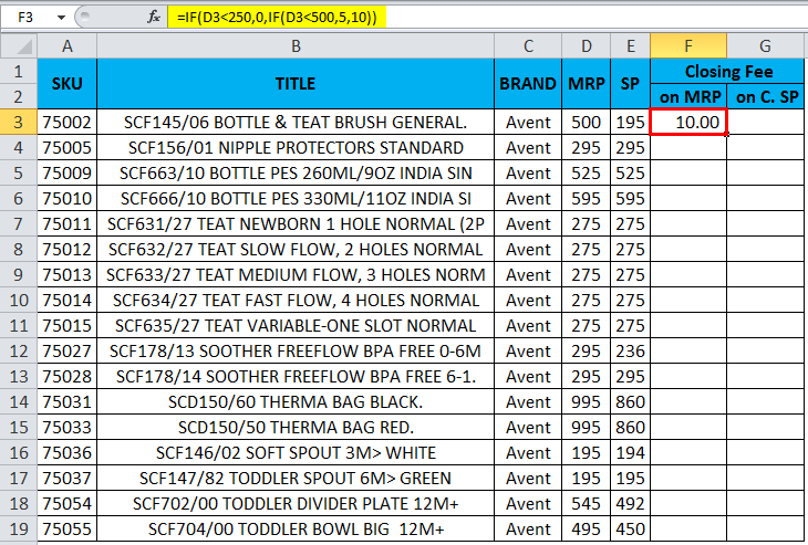
The screenshot above shows that the closing fee for MRP is 10.
How did we arrive at this value?
- First, Excel evaluated the first IF condition, which checks if 500 is less than 250. Since this is false, the condition does not apply, and Excel moves on to the next IF condition.
- The second IF condition checks if the MRP value is less than 500. In this case, the MRP is 500, which is not less than 500, so Excel moves to the last part of the IF statement, which displays the closing fee as 10.
To calculate the closing fee for the Selling Price column, we can apply another Multiple IF statement as follows: =IF(E3<250,0,IF(E3<500,5,10)).
We can then drag this formula down to all cells in the column to obtain the corresponding closing fees
The resulting table is shown below.
Things to Remember
- When we use a string in excel, Multiple IFS makes sure that we always enter the text in double quotes, or else the statement will throw the error as #NAME?
- While using Multiple IFS, make sure that we have closed multiple opening and closing parenthesis, or else we will get the error alert stating that the formula applied is wrong.
- One can include up to 127 pairs of conditions and values in the Multiple IFS function.
- Conditions in the Multiple IFS function are evaluated in their order of listing. One must arrange the conditions in accordance with the order required. In case of multiple simultaneously true conditions, the first condition in the list will take precedence.
- Multiple IFS function is only available in Excel 2016 and later versions, including Excel for Microsoft 365. In the case of an earlier version of Excel, one can use the nested IF function as an alternative.
Frequently Asked Questions(FAQs)
Q1. What is the syntax for multiple IFS functions in Excel?
Answer: The syntax for multiple IFS functions in Excel is:
=IFS(condition1,result1,condition2,result2,…,condition_n,result_n)
Q2. Can I use multiple IFS functions within a single formula in Excel?
Answer: Yes, it is possible to use multiple IFS functions within a single formula in Excel to test for different conditions and return different results.
Example:
=IFS(A1<10, “Low”, A1<20, “Medium”, A1<30, “High”, A1<40, “Very High”)
In this example, the formula checks the value in cell A1 and gives different results based on the value. If A1 is less than 10, the formula returns “Low” and if A1 is between 10 and 19, it shows “Medium“. If A1 is between 20 and 29, it shows “High“. And if A1 is between 30 and 39, it returns “Very High“. The formula shows an empty cell if none of the conditions are true.
Q3. What is the difference between multiple IFS functions and nested IF functions in Excel?
Answer: The main difference between multiple IFS functions and nested IF functions in Excel is that multiple IFS functions allow you to test for multiple conditions in a single function, while nested IF functions only allow you to test for one condition at a time.
Example of a formula using the multiple IFS function:
=IFS(A1<10,”Low”,A1<20,”Medium”,A1<30,”High”,A1>=30,”Very High”)
Example of a formula using the nested IF function:
=IF(A1<10,”Low”,IF(A1<20,”Medium”,IF(A1<30,”High”,”Very High”)))
Recommended Articles
This article has been a guide to Multiple IFS in Excel. Here we discuss the usage of Multiple IFS in Excel, practical examples, and a downloadable excel template. You can also go through our other suggested articles:
- IFERROR with VLOOKUP in Excel
- Fill Handle in Excel
- Remove Duplicates in Excel
- Excel Data Validation
I received a lot of questions on how to use IF function with 3 conditions, so I’ve decided to write an article on this topic.
The IF examples described in this article assume that you have a basic understanding of how the IF function works. All examples from this article work in Excel for Microsoft 365 or Excel 2021, 2019, 2016, 2013, 2010, and 2007.
IF is one of the most used Excel functions. In case you are unfamiliar with the IF function, then I strongly recommend reading my article on Excel IF function first. It’s a step-by-step guide, and it includes a lot of useful examples. It also shows the basics of writing an Excel IF statement with multiple conditions, but it’s not as detailed as this guide. Make sure you also download the exercise file.
As a data analyst, you need to be able to evaluate multiple conditions at the same time and perform an action or display certain values when the logical tests are TRUE. This means that you will need to learn how to write more complex formulas, which sooner or later will include multiple IF statements in Excel, nested one inside the other.
Let’s take a look at how to write a simple IF function with 3 logical tests.
The first example uses an IF statement with three OR conditions. We will use an IF formula which sets the Finance division name if the department is Accounting, Financial Reporting, or Planning & Budgeting.
The IF statement from cell E31 is:=IF(OR(D31="Accounting", D31="Financial Reporting", D31="Planning & Budgeting"), "Finance", "Other")

This IF formula works by checking three OR conditions:
- Is the data from the cell
D31equal toAccounting? In our case, the answer is no, and the formula continues and evaluates the second condition. - Is the text from the cell
D31equal toFinancial Reporting? The answer is still no, and the formula continues and evaluates the third condition. - Is the text from the cell
D31equal toPlanning & Reporting? The answer is yes, our IF function returns TRUE, and displays the word Finance in cell E31.
Next, we focus our attention on an example that uses an IF statement with three AND conditions.
Our table shows exam scores for three exams. If the student received a score of at least 70 for all three exams, then we will return Pass. Otherwise, we will display Fail.
The IF statement from cell H53 is:=IF(AND(E53>=70, F53>=70, G53>=70), "Pass", "Fail")

This IF formula works by checking all three AND conditions:
- Is the score for Exam 1
higher than or equal to 70? In our case, the answer is yes, and the formula continues and evaluates the second condition. - Is the score for Exam 2
higher than or equal to 70? Well, yes it is. Now the formula moves to the third condition. - Is the score for Exam 3 higher than or equal to 70? Yes, it is. Since all three conditions are met, the IF statement is TRUE and returns the word Pass in cell H53.
Excel IF statement with multiple conditions
The final section of this article is focused on how to write an Excel IF statement with multiple conditions, and it includes two examples:
- multiple nested IF statements (also known as nested IFS)
- formula with a mix of AND, OR, and NOT conditions
How many IF statements can you nest in Excel? The answer is 64, but I’ve never seen a formula that uses that many. Also, I’m sure that there are far better alternatives to using such a complicated formula.
Multiple nested IF statements
In this example, I have calculated the grade of the students based on their scores using a formula with 4 nested IF functions.
=IF(E107<60, "F", IF(E107<70, "D", IF(E107<80, "C", IF(E107<90, "B" ,"A"))))
Note: In this case, the order of the conditions influences the result of your formula. When your conditions overlap, Excel will return the [value_if_true] argument from the first IF statement that is TRUE and ignores the rest of the values. If you want your formula to work properly, always pay attention to the logical flow and the order of your nested IF functions.
If you have to write an IF statement with 3 outcomes, then you only need to use one nested IF function. The first IF statement will handle the first outcome, while the second one will return the second and the third possible outcomes.

Note: If you have Office 365 installed, then you can also use the new IFS function. You can read more about IFS on Microsoft’s website.
Multiple IF statements in Excel with AND, OR, and NOT conditions
I have saved the best for last. This example is the most advanced from this article, as it involves an IF statement with several other logical functions.
In the exercise file, I have included a list of orders. Each row includes the order date, the order value, the product category, and the free shipping flag. We want to flag orders as eligible if the following cumulative logical conditions are met:
- the order was placed during
2020 - the order includes products from only two categories:
PCorLaptop - the order was
notflagged asFree shipping
The formula I’ve used for cell H80 is shown below:
=IF(AND(D80>=DATE(2020,1,1), D80<=DATE(2020,12,31), OR(F80="PC", F80="Laptop"), NOT(G80="Yes")), "Eligible", "Not eligible")

Here’s how this works:
ANDmakes sure that all the logical conditions need to be met to flag the order as Eligible. If any of them is FALSE, then our entire IF statement will return the [value_if_false] argument.D80>=DATE(2020,1,1)andD80<=DATE(2020,12,31)check if the order was placed between January 1st and December 31st, 2020.ORis used to check whether the product category isPCorLaptop.- Finally,
NOTis used to check if the Free shipping flag is different fromYes.
I’ve also added a video that shows how to nest IF functions in case you are still having difficulties understanding how a nested IF formula works.
And there you have it. I hope that after reading this guide, you have a much better understanding of using IF function with 3 logical tests (or any number actually). While it may seem intimidating at first, I guarantee that if you write an IF formula with multiple criteria daily, your productivity will eventually skyrocket.
This is why, if you have any questions on how to use IF function with 3 conditions, please leave a comment below and I will do my best to help you out. I reply to every comment or email that I receive.