
The IF function allows you to make a logical comparison between a value and what you expect by testing for a condition and returning a result if that condition is True or False.
-
=IF(Something is True, then do something, otherwise do something else)
But what if you need to test multiple conditions, where let’s say all conditions need to be True or False (AND), or only one condition needs to be True or False (OR), or if you want to check if a condition does NOT meet your criteria? All 3 functions can be used on their own, but it’s much more common to see them paired with IF functions.
Use the IF function along with AND, OR and NOT to perform multiple evaluations if conditions are True or False.
Syntax
-
IF(AND()) — IF(AND(logical1, [logical2], …), value_if_true, [value_if_false]))
-
IF(OR()) — IF(OR(logical1, [logical2], …), value_if_true, [value_if_false]))
-
IF(NOT()) — IF(NOT(logical1), value_if_true, [value_if_false]))
|
Argument name |
Description |
|
|
logical_test (required) |
The condition you want to test. |
|
|
value_if_true (required) |
The value that you want returned if the result of logical_test is TRUE. |
|
|
value_if_false (optional) |
The value that you want returned if the result of logical_test is FALSE. |
|
Here are overviews of how to structure AND, OR and NOT functions individually. When you combine each one of them with an IF statement, they read like this:
-
AND – =IF(AND(Something is True, Something else is True), Value if True, Value if False)
-
OR – =IF(OR(Something is True, Something else is True), Value if True, Value if False)
-
NOT – =IF(NOT(Something is True), Value if True, Value if False)
Examples
Following are examples of some common nested IF(AND()), IF(OR()) and IF(NOT()) statements. The AND and OR functions can support up to 255 individual conditions, but it’s not good practice to use more than a few because complex, nested formulas can get very difficult to build, test and maintain. The NOT function only takes one condition.

Here are the formulas spelled out according to their logic:
|
Formula |
Description |
|---|---|
|
=IF(AND(A2>0,B2<100),TRUE, FALSE) |
IF A2 (25) is greater than 0, AND B2 (75) is less than 100, then return TRUE, otherwise return FALSE. In this case both conditions are true, so TRUE is returned. |
|
=IF(AND(A3=»Red»,B3=»Green»),TRUE,FALSE) |
If A3 (“Blue”) = “Red”, AND B3 (“Green”) equals “Green” then return TRUE, otherwise return FALSE. In this case only the first condition is true, so FALSE is returned. |
|
=IF(OR(A4>0,B4<50),TRUE, FALSE) |
IF A4 (25) is greater than 0, OR B4 (75) is less than 50, then return TRUE, otherwise return FALSE. In this case, only the first condition is TRUE, but since OR only requires one argument to be true the formula returns TRUE. |
|
=IF(OR(A5=»Red»,B5=»Green»),TRUE,FALSE) |
IF A5 (“Blue”) equals “Red”, OR B5 (“Green”) equals “Green” then return TRUE, otherwise return FALSE. In this case, the second argument is True, so the formula returns TRUE. |
|
=IF(NOT(A6>50),TRUE,FALSE) |
IF A6 (25) is NOT greater than 50, then return TRUE, otherwise return FALSE. In this case 25 is not greater than 50, so the formula returns TRUE. |
|
=IF(NOT(A7=»Red»),TRUE,FALSE) |
IF A7 (“Blue”) is NOT equal to “Red”, then return TRUE, otherwise return FALSE. |
Note that all of the examples have a closing parenthesis after their respective conditions are entered. The remaining True/False arguments are then left as part of the outer IF statement. You can also substitute Text or Numeric values for the TRUE/FALSE values to be returned in the examples.
Here are some examples of using AND, OR and NOT to evaluate dates.

Here are the formulas spelled out according to their logic:
|
Formula |
Description |
|---|---|
|
=IF(A2>B2,TRUE,FALSE) |
IF A2 is greater than B2, return TRUE, otherwise return FALSE. 03/12/14 is greater than 01/01/14, so the formula returns TRUE. |
|
=IF(AND(A3>B2,A3<C2),TRUE,FALSE) |
IF A3 is greater than B2 AND A3 is less than C2, return TRUE, otherwise return FALSE. In this case both arguments are true, so the formula returns TRUE. |
|
=IF(OR(A4>B2,A4<B2+60),TRUE,FALSE) |
IF A4 is greater than B2 OR A4 is less than B2 + 60, return TRUE, otherwise return FALSE. In this case the first argument is true, but the second is false. Since OR only needs one of the arguments to be true, the formula returns TRUE. If you use the Evaluate Formula Wizard from the Formula tab you’ll see how Excel evaluates the formula. |
|
=IF(NOT(A5>B2),TRUE,FALSE) |
IF A5 is not greater than B2, then return TRUE, otherwise return FALSE. In this case, A5 is greater than B2, so the formula returns FALSE. |

Using AND, OR and NOT with Conditional Formatting
You can also use AND, OR and NOT to set Conditional Formatting criteria with the formula option. When you do this you can omit the IF function and use AND, OR and NOT on their own.
From the Home tab, click Conditional Formatting > New Rule. Next, select the “Use a formula to determine which cells to format” option, enter your formula and apply the format of your choice.

Using the earlier Dates example, here is what the formulas would be.

|
Formula |
Description |
|---|---|
|
=A2>B2 |
If A2 is greater than B2, format the cell, otherwise do nothing. |
|
=AND(A3>B2,A3<C2) |
If A3 is greater than B2 AND A3 is less than C2, format the cell, otherwise do nothing. |
|
=OR(A4>B2,A4<B2+60) |
If A4 is greater than B2 OR A4 is less than B2 plus 60 (days), then format the cell, otherwise do nothing. |
|
=NOT(A5>B2) |
If A5 is NOT greater than B2, format the cell, otherwise do nothing. In this case A5 is greater than B2, so the result will return FALSE. If you were to change the formula to =NOT(B2>A5) it would return TRUE and the cell would be formatted. |
Note: A common error is to enter your formula into Conditional Formatting without the equals sign (=). If you do this you’ll see that the Conditional Formatting dialog will add the equals sign and quotes to the formula — =»OR(A4>B2,A4<B2+60)», so you’ll need to remove the quotes before the formula will respond properly.
Need more help?

See also
You can always ask an expert in the Excel Tech Community or get support in the Answers community.
Learn how to use nested functions in a formula
IF function
AND function
OR function
NOT function
Overview of formulas in Excel
How to avoid broken formulas
Detect errors in formulas
Keyboard shortcuts in Excel
Logical functions (reference)
Excel functions (alphabetical)
Excel functions (by category)
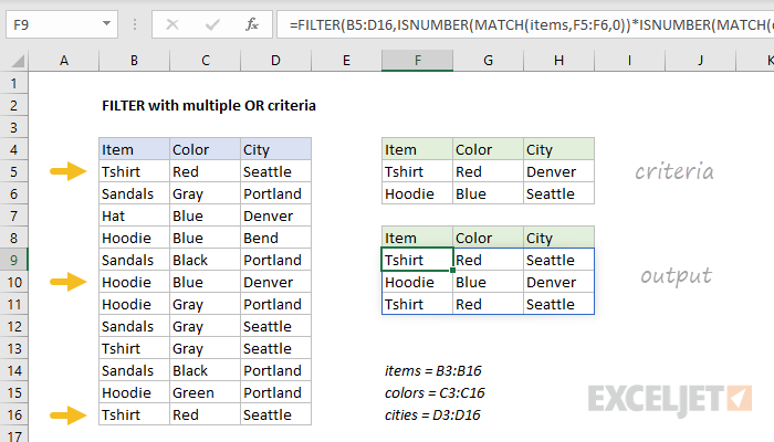
In this example, criteria are entered in the range F5:H6. The logic of the formula is:
item is (tshirt OR hoodie) AND color is (red OR blue) AND city is (denver OR seattle)
The filtering logic of this formula (the include argument) is applied with the ISNUMBER and MATCH functions, together with boolean logic applied in an array operation.
MATCH is configured «backwards», with lookup_values coming from the data, and criteria used for the lookup_array. For example, the first condition is that items must be either a Tshirt or Hoodie. To apply this condition, MATCH is set up like this:
MATCH(items,F5:F6,0) // check for tshirt or hoodie
Because there are 12 values in the data, the result is an array with 12 values like this:
{1;#N/A;#N/A;2;#N/A;2;2;#N/A;1;#N/A;2;1}
This array contains either #N/A errors (no match) or numbers (match). Notice numbers correspond to items that are either Tshirt or Hoodie. To convert this array into TRUE and FALSE values, the MATCH function is wrapped in the ISNUMBER function:
ISNUMBER(MATCH(items,F5:F6,0))
which yields an array like this:
{TRUE;FALSE;FALSE;TRUE;FALSE;TRUE;TRUE;FALSE;TRUE;FALSE;TRUE;TRUE}
In this array, the TRUE values correspond to tshirt or hoodie.
The full formula contains three expressions like the above used for the include argument of the FILTER function:
ISNUMBER(MATCH(items,F5:F6,0))* // tshirt or hoodie
ISNUMBER(MATCH(colors,G5:G6,0))* // red or blue
ISNUMBER(MATCH(cities,H5:H6,0))) // denver or seattle
After MATCH and ISNUMBER are evaluated, we have three arrays containing TRUE and FALSE values. The math operation of multiplying these arrays together coerces the TRUE and FALSE values to 1s and 0s, so we can visualize the arrays at this point like this:
{1;0;0;1;0;1;1;0;1;0;1;1}*
{1;0;1;1;0;1;0;0;0;0;0;1}*
{1;0;1;0;0;1;0;1;1;0;0;1}
The result, following the rules of boolean arithmetic, is a single array:
{1;0;0;0;0;1;0;0;0;0;0;1}
which becomes the include argument in the FILTER function:
=FILTER(B5:D16,{1;0;0;0;0;1;0;0;0;0;0;1})
The final result is the three rows of data shown in F9:H11
With hard-coded values
Although the formula in the example uses criteria entered directly on the worksheet, criteria can be hard-coded as array constants instead like this:
=FILTER(B5:D16,
ISNUMBER(MATCH(items,{"Tshirt";"Hoodie"},0))*
ISNUMBER(MATCH(colors,{"Red";"Blue"},0))*
ISNUMBER(MATCH(cities,{"Denver";"Seattle"},0)))
Logical functions perform criteria-based calculations in Excel. To match single criteria, we can use the IF logical condition. Having to perform multiple tests, we can use nested IF conditions. But imagine the situation of matching multiple criteria to arrive at a single result is the complex criteria-based calculation. To compare various criteria in Excel, one needs to be an advanced user of functions in Excel.
Matching multiple conditions is possible to perform by using multiple logical conditions. This article will take you through matching multiple criteria in Excel.
Table of contents
- Match Multiple Criteria in Excel
- How to Match Multiple Criteria Excel? (Examples)
- Example #1 – Logical Functions in Excel
- Example #2 – Multiple Logical Functions in Excel
- Things to Remember
- Recommended Articles
- How to Match Multiple Criteria Excel? (Examples)
How to Match Multiple Criteria Excel? (Examples)
You can download this Match Multiple Criteria Excel Template here – Match Multiple Criteria Excel Template
Example #1 – Logical Functions in Excel
Commonly, we use three logical functions in Excel to perform multiple criteria calculations. The three functions are IF, AND, and OR conditions.
For example, let us look at the calculation below of the AND formula.

Look at the formula below; we have tested whether the cell A1 value is >20 or not, the B1 cell value is >20 or not, and the C1 cell value is >20.
In the above function, all the cell values are >20, so the result is “TRUE.” We will change one of the cell values to less than 20.

The B1 cell value changed to 18, less than 20, so the result is “FALSE,” even though the other two cell values are >20.
We will apply the OR function in excelThe OR function in Excel is used to test various conditions, allowing you to compare two values or statements in Excel. If at least one of the arguments or conditions evaluates to TRUE, it will return TRUE. Similarly, if all of the arguments or conditions are FALSE, it will return FASLE.read more for the same number.

For the OR function, one criterion needs to be satisfied to get the result as “TRUE.” So we need all the conditions to meet the “TRUE” result, unlike the AND function.
Example #2 – Multiple Logical Functions in Excel
Now, we will see how to perform multiple logical functions to match multiple conditions.
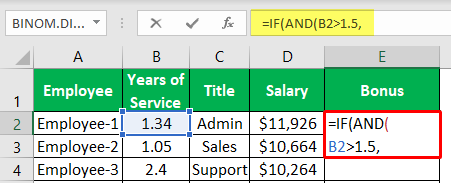
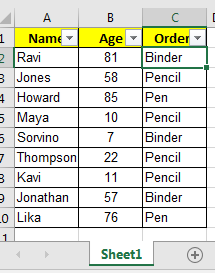
- Let us look at the below data in Excel.

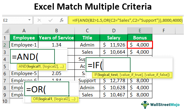
We need to calculate the “Bonus” amount based on the below conditions from the above data.
If the “Year of Service” is >1.5 years and if the “Department” is “Sales” or “Support,” then the bonus is $8,000; otherwise, the bonus will be $4,000.
So, to arrive at one result, we need to match multiple criteria in Excel. In this case, we need to test whether the “Year of Service” is 1.5 and whether the “Department” is “Sales” or “Support” to arrive at the bonus amount.
- We must first open the condition in Excel.

- The first logical condition to test is compulsory, whether the year of service is >1.5 years or not. So for the mandatory “TRUE” result, we need to use AND function.
The above logical test will return “TRUE” only if the year of service is >1.5. Otherwise, we will get “FALSE” as a result. Inside this AND function, we need to test one more criterion, i.e., whether the “Department” is “Sales” or “Support,” to arrive at a bonus amount.
- If any department matches these criteria, we need the “TRUE” result, so we need to use the OR function.

As you can see above, we have used AND and OR functions to match single criteria. So, for example, the AND function will test the year of service at>1.5 years, and the OR function will test whether the department is “Sales” or “Support.” So if the “Year of Service” is 1.5 and the department is either “Sales” or “Support,” the logical test result will be “TRUE” or else “FALSE.”
- If the logical test is “TRUE,” we need the bonus amount at $8,000. So for the value, if True argument, we need to supply #8,000.

- If the logical test is “FALSE,” we need the bonus amount at $4,000.

- So, we are done with applying the formula, closing the formula, and applying the formula to other cells to get the result in other cells.

Now, let us look at the fourth row. In this case, the “Year of Service” is 2.4, and the “Department” is “Support,” so the bonus arrives at $8,000. Like this, we can match multiple criteria in Excel.
Things to Remember
- To test multiple criteria to arrive at a single result, we need to use multiple logical functions inside the IF condition.
- The AND and OR Excel functions are the two supporting functions we can use to test multiple criteria.
- The AND function in Excel may return “TRUE” only if all the logical tests are satisfied, but on the other hand, the OR function requires at least one logical test to be met to get a “TRUE” result.
Recommended Articles
This article has been a guide to Excel Match Multiple Criteria. Here, we discuss matching multiple criteria in Excel using AND, IF, and OR formulas and practical examples. You may learn more about Excel from the following articles: –
- Excel Break-Even Analysis
- Match Function Excel Examples
- VLOOKUP with Multiple Criteria
- SUMPRODUCT with Multiple Criteria
- NETWORKDAYS Excel Function
Содержание
- FILTER with multiple OR criteria
- Related functions
- Summary
- Explanation
- With hard-coded values
- How to apply multiple filtering criteria by combining AND and OR operations with the FILTER() function in Excel
- Account Information
- Share with Your Friends
- How to apply multiple filtering criteria by combining AND and OR operations with the FILTER() function in Excel
- Must-read Windows coverage
- The operations
- How to use the built-in filter in Excel
- How to use * in Excel
- How to use + in Excel
- And more
- Microsoft Weekly Newsletter
- Filter by using advanced criteria
- Overview of advanced filter criteria
- Sample data
- Comparison operators
- Using the equal sign to type text or a value
- Considering case-sensitivity
- Using pre-defined names
- Creating criteria by using a formula
- Multiple criteria, one column, any criteria true
- Multiple criteria, multiple columns, all criteria true
- Multiple criteria, multiple columns, any criteria true
- Multiple sets of criteria, one column in all sets
- Multiple sets of criteria, multiple columns in each set
- Wildcard criteria
FILTER with multiple OR criteria
Summary
To extract data with multiple OR conditions, you can use the FILTER function together with the MATCH function. In the example shown, the formula in F9 is:
where items (B3:B16), colors (C3:C16), and cities (D3:D16) are named ranges.
This formula returns data where item is (tshirts OR hoodie) AND color is (red OR blue) AND city is (denver OR seattle).
Explanation
In this example, criteria are entered in the range F5:H6. The logic of the formula is:
item is (tshirt OR hoodie) AND color is (red OR blue) AND city is (denver OR seattle)
The filtering logic of this formula (the include argument) is applied with the ISNUMBER and MATCH functions, together with boolean logic applied in an array operation.
MATCH is configured «backwards», with lookup_values coming from the data, and criteria used for the lookup_array. For example, the first condition is that items must be either a Tshirt or Hoodie. To apply this condition, MATCH is set up like this:
Because there are 12 values in the data, the result is an array with 12 values like this:
This array contains either #N/A errors (no match) or numbers (match). Notice numbers correspond to items that are either Tshirt or Hoodie. To convert this array into TRUE and FALSE values, the MATCH function is wrapped in the ISNUMBER function:
which yields an array like this:
In this array, the TRUE values correspond to tshirt or hoodie.
The full formula contains three expressions like the above used for the include argument of the FILTER function:
After MATCH and ISNUMBER are evaluated, we have three arrays containing TRUE and FALSE values. The math operation of multiplying these arrays together coerces the TRUE and FALSE values to 1s and 0s, so we can visualize the arrays at this point like this:
The result, following the rules of boolean arithmetic, is a single array:
which becomes the include argument in the FILTER function:
The final result is the three rows of data shown in F9:H11
With hard-coded values
Although the formula in the example uses criteria entered directly on the worksheet, criteria can be hard-coded as array constants instead like this:
Источник
How to apply multiple filtering criteria by combining AND and OR operations with the FILTER() function in Excel
Account Information
How to apply multiple filtering criteria by combining AND and OR operations with the FILTER() function in Excel
How to apply multiple filtering criteria by combining AND and OR operations with the FILTER() function in Excel
Learn a seemingly tricky way to extract data from your Microsoft Excel spreadsheet.
We may be compensated by vendors who appear on this page through methods such as affiliate links or sponsored partnerships. This may influence how and where their products appear on our site, but vendors cannot pay to influence the content of our reviews. For more info, visit our Terms of Use page.  Image: 200dgr/Shutterstock
Applying multiple criteria against different columns to filter the data set in Microsoft Excel sounds difficult but it really isn’t as hard as it sounds. The most important part is to get the logic between those columns right. For instance, do you want to see all records where one column equals x and another equals y? Or you might want to see all records where one column = x or another column equals y. The results will be very different. In this article, I’ll show you how to include AND and OR operations in Excel’s FILTER() function.
Must-read Windows coverage
In several spots, you’ll read “AND and OR,” which is grammatically awkward. I’m referring to the AND and OR operations generically. We won’t be using the AND() and OR() functions. I’ll use uppercase only to improve readability.
I’m using Microsoft 365 on a Windows 10 64-bit system. The FILTER() function is available in Microsoft 365, Excel Online, Excel 2021, Excel for iPad and iPhone and Excel for Android tablets and phones. I recommend that you wait to upgrade to Windows 11 until all the kinks are worked out. For your convenience, you can download the demonstration .xlsx file.
The operations
The logic operators * and + specify a relationship between the operands in an expression (AND and OR, respectively). Specifically, * (AND) requires that both operands must be true to return true. On the other hand, + (OR) requires that only one operand be true to return true. In our case, operand is a simple expression. For instance
1 + 3 = 4 AND 2 + 1 = 3
returns true while
1 + 3 = 2 AND 2 + 1 = 3
returns false. If we apply the OR operation to the same expressions
1 + 3 = 4 OR 2 + 1 = 3
returns true because at least one expression is true and
1 + 3 = 2 AND 2 + 1 = 3
returns true for the same reason.
Now let’s work through some examples.
How to use the built-in filter in Excel
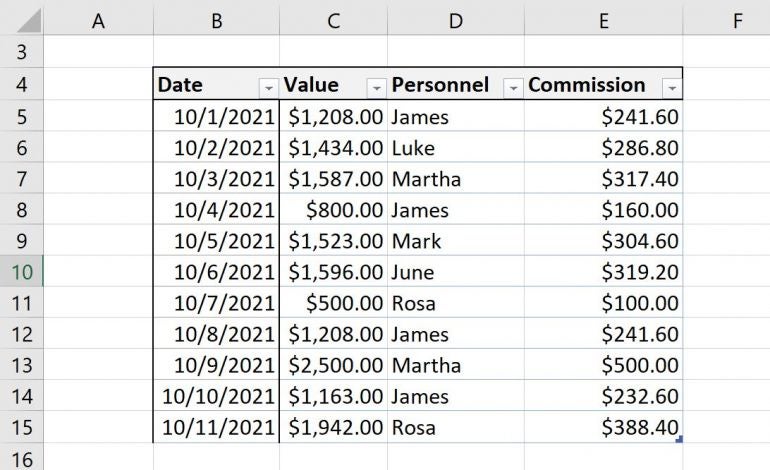
Let’s suppose that you track commissions using the simple data set shown in Figure A. Furthermore, you want to know if anyone is falling below a specific benchmark—say, $200. Fortunately, for users who know how to use the built-in filters, you don’t even need the FILTER() function. However, using the built-in feature works on the source data, and it’s difficult to reference in other expressions, so while it’s easy, it might not be the right solution for every situation.
Figure A
 Use the built-in filters.
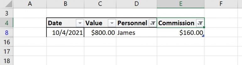
We have two criteria, personnel and commission. Let’s use a built-in feature to see the filtered set for James with any commission less than or equal to $200, keeping in mind that you must be working with a Table object:
- Click the Personnel dropdown, uncheck (Select All), check James, and click OK. Doing so will display four records.
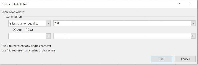
- From the Commission dropdown, choose Number Filters and then choose Less Than Or Equal To, as shown in Figure B.
- Enter 200 in the control to the right of the comparison operator (Figure C) and click OK.
Figure B
 Choose a built-in filter.
Figure C
 Enter the benchmark amount.
As you can see in Figure D, James has only one commission that falls below the $200 benchmark: $160.
Figure D
 The built-in filter feature can handle criteria across multiple columns.
It’s easy but does require a bit of knowledge about how the feature works. On the other hand, the feature works with the data source, and that might not be what you want.
How to use * in Excel
You might have noticed (Figure C) the AND and OR options in the dialog where you entered the benchmark amount. This option allows you to enter other criteria for the same column—Commission. To accomplish an AND across multiple columns, we’ll use the * symbol, which is similar to the AND() function, but AND() doesn’t work as you might expect when combined with FILTER().
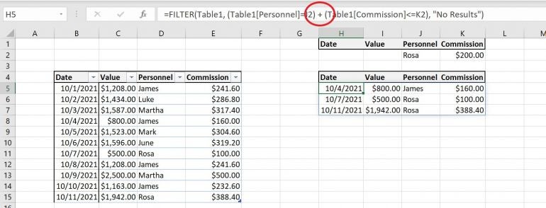
Figure E shows the results of entering the following function
=FILTER(Table1, (Table1[Personnel]=J2) * (Table1[Commission]  Change the name in J2 or the amount in K2 to update the result set.
The * character does a great job of allowing us to apply criteria across multiple rows. But what about OR?
How to use + in Excel
Sometimes, you’ll want to check for the existence of one value or another. When that’s the case, use the + symbol. We can see the difference quickly enough by modifying the function in H5: Replace the * symbol with the + symbol. As you can see in Figure G, there are three records that match the criteria. The personnel value is James, or the commission value is less than or equal to 200.
Figure G
 Three records match the criteria.
And more
In these simple examples, I worked with only two columns, but it’s no problem to add more. When you do, the parentheses become very important. For example, let’s suppose you want to add another person to the personnel criteria, such as Rosa—you want to match any record where James or Rosa has a commission value less than 200. Again, it’s a simple edit to the original function:
- Select H5.
- Enter (Table1[Personnel]=J3) * between the first and second expressions for the second argument (Figure H). Wrap the first two expression in parentheses: ((Table1[Personnel]=J2) + (Table1[Personnel]=J3)) * (Table1[Commission]
 Modify the function in H5.
 Modify the function in H5.
 Figure I
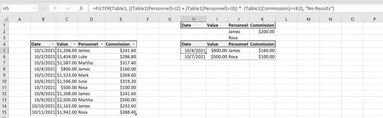 This function returns two records.
There are two records for James or Rosa where the commission is less than or equal to 200 (and). To include even more personnel, enter more rows and modify the function by adding a new expression, and remember that entire OR needs to be wrapped in parentheses. The same would be true if you were referencing multiple expressions on the other side. Wrap multiple AND expressions together and wrap multiple OR expressions together.

Microsoft Weekly Newsletter
Be your company’s Microsoft insider by reading these Windows and Office tips, tricks, and cheat sheets.
Источник
Filter by using advanced criteria
If the data you want to filter requires complex criteria (such as Type = «Produce» OR Salesperson = «Davolio»), you can use the Advanced Filter dialog box.
To open the Advanced Filter dialog box, click Data > Advanced.

Salesperson = «Davolio» OR Salesperson = «Buchanan»
Type = «Produce» AND Sales > 1000
Type = «Produce» OR Salesperson = «Buchanan»
(Sales > 6000 AND Sales 3000) OR
(Salesperson = «Buchanan» AND Sales > 1500)
Salesperson = a name with ‘u’ as the second letter
Overview of advanced filter criteria
The Advanced command works differently from the Filter command in several important ways.
It displays the Advanced Filter dialog box instead of the AutoFilter menu.
You type the advanced criteria in a separate criteria range on the worksheet and above the range of cells or table that you want to filter. Microsoft Office Excel uses the separate criteria range in the Advanced Filter dialog box as the source for the advanced criteria.
Sample data
The following sample data is used for all procedures in this article.
The data includes four blank rows above the list range that will be used as a criteria range (A1:C4) and a list range (A6:C10). The criteria range has column labels and includes at least one blank row between the criteria values and the list range.
To work with this data, select it in the following table, copy it, and then paste it in cell A1 of a new Excel worksheet.
Comparison operators
You can compare two values by using the following operators. When two values are compared by using these operators, the result is a logical value—either TRUE or FALSE.
> (greater than sign)
= (greater than or equal to sign)
Greater than or equal to
(not equal to sign)
Using the equal sign to type text or a value
Because the equal sign ( =) is used to indicate a formula when you type text or a value in a cell, Excel evaluates what you type; however, this may cause unexpected filter results. To indicate an equality comparison operator for either text or a value, type the criteria as a string expression in the appropriate cell in the criteria range:
Where entry is the text or value you want to find. For example:
What you type in the cell
What Excel evaluates and displays
Considering case-sensitivity
When filtering text data, Excel doesn’t distinguish between uppercase and lowercase characters. However, you can use a formula to perform a case-sensitive search. For an example, see the section Wildcard criteria.
Using pre-defined names
You can name a range Criteria, and the reference for the range will appear automatically in the Criteria range box. You can also define the name Database for the list range to be filtered and define the name Extract for the area where you want to paste the rows, and these ranges will appear automatically in the List range and Copy to boxes, respectively.
Creating criteria by using a formula
You can use a calculated value that is the result of a formula as your criterion. Remember the following important points:
The formula must evaluate to TRUE or FALSE.
Because you are using a formula, enter the formula as you normally would, and do not type the expression in the following way:
Do not use a column label for criteria labels; either keep the criteria labels blank or use a label that is not a column label in the list range (in the examples that follow, Calculated Average and Exact Match).
If you use a column label in the formula instead of a relative cell reference or a range name, Excel displays an error value such as #NAME? or #VALUE! in the cell that contains the criterion. You can ignore this error because it does not affect how the list range is filtered.
The formula that you use for criteria must use a relative reference to refer to the corresponding cell in the first row of data.
All other references in the formula must be absolute references.
Multiple criteria, one column, any criteria true
Boolean logic: (Salesperson = «Davolio» OR Salesperson = «Buchanan»)
Insert at least three blank rows above the list range that can be used as a criteria range. The criteria range must have column labels. Make sure that there is at least one blank row between the criteria values and the list range.
To find rows that meet multiple criteria for one column, type the criteria directly below each other in separate rows of the criteria range. Using the example, enter:
Click a cell in the list range. Using the example, click any cell in the range A6:C10.
On the Data tab, in the Sort & Filter group, click Advanced.
Do one of the following:
To filter the list range by hiding rows that don’t match your criteria, click Filter the list, in-place.
To filter the list range by copying rows that match your criteria to another area of the worksheet, click Copy to another location, click in the Copy to box, and then click the upper-left corner of the area where you want to paste the rows.
Tip When you copy filtered rows to another location, you can specify which columns to include in the copy operation. Before filtering, copy the column labels for the columns that you want to the first row of the area where you plan to paste the filtered rows. When you filter, enter a reference to the copied column labels in the Copy to box. The copied rows will then include only the columns for which you copied the labels.
In the Criteria range box, enter the reference for the criteria range, including the criteria labels. Using the example, enter $A$1:$C$3.
To move the Advanced Filter dialog box out of the way temporarily while you select the criteria range, click Collapse Dialog  .
.
Using the example, the filtered result for the list range is:
Multiple criteria, multiple columns, all criteria true
Boolean logic: (Type = «Produce» AND Sales > 1000)
Insert at least three blank rows above the list range that can be used as a criteria range. The criteria range must have column labels. Make sure that there is at least one blank row between the criteria values and the list range.
To find rows that meet multiple criteria in multiple columns, type all the criteria in the same row of the criteria range. Using the example, enter:
Click a cell in the list range. Using the example, click any cell in the range A6:C10.
On the Data tab, in the Sort & Filter group, click Advanced.
Do one of the following:
To filter the list range by hiding rows that don’t match your criteria, click Filter the list, in-place.
To filter the list range by copying rows that match your criteria to another area of the worksheet, click Copy to another location, click in the Copy to box, and then click the upper-left corner of the area where you want to paste the rows.
Tip When you copy filtered rows to another location, you can specify which columns to include in the copy operation. Before filtering, copy the column labels for the columns that you want to the first row of the area where you plan to paste the filtered rows. When you filter, enter a reference to the copied column labels in the Copy to box. The copied rows will then include only the columns for which you copied the labels.
In the Criteria range box, enter the reference for the criteria range, including the criteria labels. Using the example, enter $A$1:$C$2.
To move the Advanced Filter dialog box out of the way temporarily while you select the criteria range, click Collapse Dialog .
Using the example, the filtered result for the list range is:
Multiple criteria, multiple columns, any criteria true
Boolean logic: (Type = «Produce» OR Salesperson = «Buchanan»)
Insert at least three blank rows above the list range that can be used as a criteria range. The criteria range must have column labels. Make sure that there is at least one blank row between the criteria values and the list range.
To find rows that meet multiple criteria in multiple columns where any criteria can be true, type the criteria in the different columns and rows of the criteria range. Using the example, enter:
Click a cell in the list range. Using the example, click any cell in the list range A6:C10.
On the Data tab, in the Sort & Filter group, click Advanced.
Do one of the following:
To filter the list range by hiding rows that don’t match your criteria, click Filter the list, in-place.
To filter the list range by copying rows that match your criteria to another area of the worksheet, click Copy to another location, click in the Copy to box, and then click the upper-left corner of the area where you want to paste the rows.
Tip: When you copy filtered rows to another location, you can specify which columns to include in the copy operation. Before filtering, copy the column labels for the columns that you want to the first row of the area where you plan to paste the filtered rows. When you filter, enter a reference to the copied column labels in the Copy to box. The copied rows will then include only the columns for which you copied the labels.
In the Criteria range box, enter the reference for the criteria range, including the criteria labels. Using the example, enter $A$1:$B$3.
To move the Advanced Filter dialog box out of the way temporarily while you select the criteria range, click Collapse Dialog .
Using the example, the filtered result for the list range is:
Multiple sets of criteria, one column in all sets
Boolean logic: ( (Sales > 6000 AND Sales
To find rows that meet multiple sets of criteria where each set includes criteria for one column, include multiple columns with the same column heading. Using the example, enter:
Click a cell in the list range. Using the example, click any cell in the list range A6:C10.
On the Data tab, in the Sort & Filter group, click Advanced.
Do one of the following:
To filter the list range by hiding rows that don’t match your criteria, click Filter the list, in-place.
To filter the list range by copying rows that match your criteria to another area of the worksheet, click Copy to another location, click in the Copy to box, and then click the upper-left corner of the area where you want to paste the rows.
Tip: When you copy filtered rows to another location, you can specify which columns to include in the copy operation. Before filtering, copy the column labels for the columns that you want to the first row of the area where you plan to paste the filtered rows. When you filter, enter a reference to the copied column labels in the Copy to box. The copied rows will then include only the columns for which you copied the labels.
In the Criteria range box, enter the reference for the criteria range, including the criteria labels. Using the example, enter $A$1:$D$3.
To move the Advanced Filter dialog box out of the way temporarily while you select the criteria range, click Collapse Dialog .
Using the example, the filtered result for the list range is:
Multiple sets of criteria, multiple columns in each set
Boolean logic: ( (Salesperson = «Davolio» AND Sales >3000) OR (Salesperson = «Buchanan» AND Sales > 1500) )
Insert at least three blank rows above the list range that can be used as a criteria range. The criteria range must have column labels. Make sure that there is at least one blank row between the criteria values and the list range.
To find rows that meet multiple sets of criteria, where each set includes criteria for multiple columns, type each set of criteria in separate columns and rows. Using the example, enter:
Click a cell in the list range. Using the example, click any cell in the list range A6:C10.
On the Data tab, in the Sort & Filter group, click Advanced.
Do one of the following:
To filter the list range by hiding rows that don’t match your criteria, click Filter the list, in-place.
To filter the list range by copying rows that match your criteria to another area of the worksheet, click Copy to another location, click in the Copy to box, and then click the upper-left corner of the area where you want to paste the rows.
Tip When you copy filtered rows to another location, you can specify which columns to include in the copy operation. Before filtering, copy the column labels for the columns that you want to the first row of the area where you plan to paste the filtered rows. When you filter, enter a reference to the copied column labels in the Copy to box. The copied rows will then include only the columns for which you copied the labels.
In the Criteria range box, enter the reference for the criteria range, including the criteria labels. Using the example, enter $A$1:$C$3.To move the Advanced Filter dialog box out of the way temporarily while you select the criteria range, click Collapse Dialog .
Using the example, the filtered result for the list range would be:
Wildcard criteria
Boolean logic: Salesperson = a name with ‘u’ as the second letter
To find text values that share some characters but not others, do one or more of the following:
Type one or more characters without an equal sign ( =) to find rows with a text value in a column that begin with those characters. For example, if you type the text Dav as a criterion, Excel finds «Davolio,» «David,» and «Davis.»
Use a wildcard character.
Any single character
For example, sm?th finds «smith» and «smyth»
Any number of characters
For example, *east finds «Northeast» and «Southeast»
(tilde) followed by ?, *, or
A question mark, asterisk, or tilde
For example, fy91
Insert at least three blank rows above the list range that can be used as a criteria range. The criteria range must have column labels. Make sure that there is at least one blank row between the criteria values and the list range.
In the rows below the column labels, type the criteria that you want to match. Using the example, enter:
Click a cell in the list range. Using the example, click any cell in the list range A6:C10.
On the Data tab, in the Sort & Filter group, click Advanced.
Do one of the following:
To filter the list range by hiding rows that don’t match your criteria, click Filter the list, in-place
To filter the list range by copying rows that match your criteria to another area of the worksheet, click Copy to another location, click in the Copy to box, and then click the upper-left corner of the area where you want to paste the rows.
Tip: When you copy filtered rows to another location, you can specify which columns to include in the copy operation. Before filtering, copy the column labels for the columns that you want to the first row of the area where you plan to paste the filtered rows. When you filter, enter a reference to the copied column labels in the Copy to box. The copied rows will then include only the columns for which you copied the labels.
In the Criteria range box, enter the reference for the criteria range, including the criteria labels. Using the example, enter $A$1:$B$3.
To move the Advanced Filter dialog box out of the way temporarily while you select the criteria range, click Collapse Dialog .
Using the example, the filtered result for the list range is:
Источник
Basically, when we supply multiple conditions to a COUNTIFS function, it checks all the conditions and returns row which matches all the conditions. Which means it runs on AND logic.
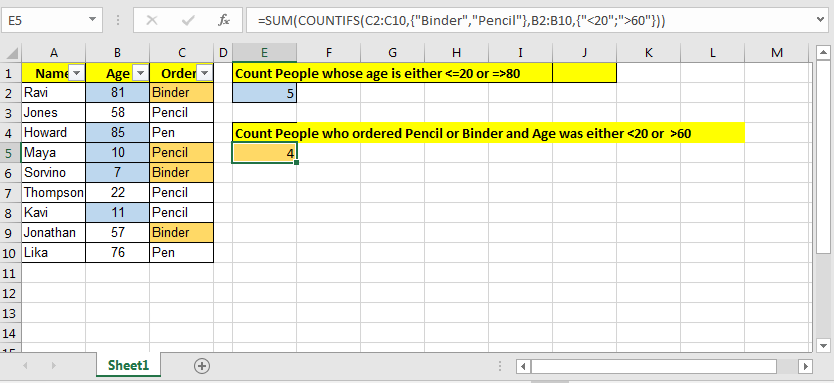
But what if you want to count on an OR logic? We need to accomplish COUNTIFS with OR logic.
This can be done easily with arrays and SUM function. Let’s see how…
Generic Formula To Countif With OR Logic For Multiple Optional Conditions
=SUM(COUNTIFS(range{condition1, condition2,…})
Example COUNTIFS with OR
So this one time, I had this data. Where I needed to count people who had aged less than or equal to 20 OR greater than or equal to 80. I did it using SUM function and arrays. Come, I’ll show you how.
So I had these two conditions (“<=20”,”>=80”). Either of them needed to be true to be counted. So I wrote this COUNTIF formula
=SUM(COUNTIFS(B2:B10,{«<=20″,»>=80″})
It gave the correct answer as 5.
How does it work?
The COUNTIFS matched each element of array {«<=20″,»>=80″} and gave count of each item in the array as {3,2}.
Now you know how SUM function in Excel works. SUM function added the values in the array(SUM({3,2}) and gives us the result 5. This crit
Let me show you another example of COUNTIFS with multiple criteria with or logic. This time I will not explain it to you. You need to figure it out.
COUNTIFS Multiple Criteria Example Part 2
Now this one is the final one. Here I had two sets of OR conditions and one AND. So the query was:
Count the people who ordered Pencil OR Binder AND Age was either 60:
It was tricky but i figured it out. Here is the formula.
=SUM(COUNTIFS(C2:C10,{«Binder»,»Pencil»},B2:B10,{«<20″;»>60″}))
This gave me the exact count of 4 for the query.
How It Worked
Actually here I used two-dimensional arrays. Note that semicolon in {«<20″;»>60″}. It adds a second dimension or says columns to the array as {1,2;1,0}.
So basically, first it finds all the binders or pencils in range C2:C10. Then in the found list, it checks who are under the age of 20 or more aged than 60.
So what you think. I used COUNTIFS to count multiple criteria with multiple conditions. First I told how I used excel countifs two criteria match and then we used countifs multiple criteria match with or logic. Don’t worry about the version of excel. It will work in Excel 2016, Excel 2013, Excel 2010 and older which have the COUNTIF function and concept of array formulas.
Related Articles:
How to COUNTIFS Two Criteria Match in Excel
How to Count Cells That Contain This Or That in Excel
How To Count Unique Text in Excel
Popular Articles:
50 Excel Shortcuts to Increase Your Productivity
How to use the VLOOKUP Function in Excel
How to use the COUNTIF function in Excel
How to use the SUMIF Function in Excel
Excel Match Multiple Criteria (Table of Contents)
- Introduction to Match Multiple Criteria in Excel
- How to Match Multiple Criteria in Excel?
Introduction to Match Multiple Criteria in Excel
As a data analyst, you always need to deal with multiple criteria and conditions to get the desired result. In Excel, you can use the IF Statement for conditional outputs. However, at times you need to construct more sophisticated logical tests in order to get the desired results. It may include the multiple IF Statements (i.e. nested IF) or can also be achieved with the help of some logical operators used under IF statements. We ideally can construct multiple criteria’s using logical AND & OR operator under the IF Statement.
- AND Operator: If you use logical AND operator/keyword under IF Statement, you will get TRUE as a result if all conditions/criteria are satisfied. Otherwise, it will return FALSE.
- OR Operator: If you use logical OR operator/keyword under IF statement, you’ll get TRUE as a result if at least one of the multiple conditions/criteria are satisfied. Else it will return FALSE.
How to Match Multiple Criteria in Excel?
To Match Multiple Criteria in Excel is very simple and easy. Let’s understand this function with some examples.
You can download this Match Multiple Criteria Excel Template here – Match Multiple Criteria Excel Template
Example #1 – AND/OR Operators Works for Multiple Criteria
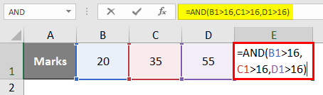
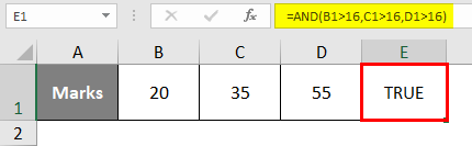
Suppose we have three sets of marks for a student as shown below:

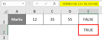
Step 1: In cell E1, as we need to check how AND operator works for multiple criteria, start initiating the formula by typing “=AND(
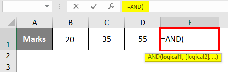
Step 2: We need to specify logical criteria under AND function. Use criteria as cell value greater than 16 for all cells (B1, C1, D1). You can use a comma as a separator to separate the multiple criteria conditions. See the screenshot below:
Once you press Enter key, you can see TRUE as a result in cell E1. Since all values present in cell B1, C1, and D1 are greater than 16, all the criteria are satisfied, leading to a Boolean output as TRUE under cell E1.
Step 3: Change the value in cell B1 as 12 and see how the result in cell E1 is affected.
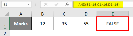
You can see with the same criteria under AND function, if we change the value under cell B1 as less than the criteria value (i.e. 16), we will get the output as FALSE. Since the value in cell B1 is not greater than 16, not all the criteria are satisfied.
Step 4: In cell E2, use the OR to check how it works; use the same criteria values. Ideally, OR gives Boolean output as TRUE if at least one of the criteria is satisfied.
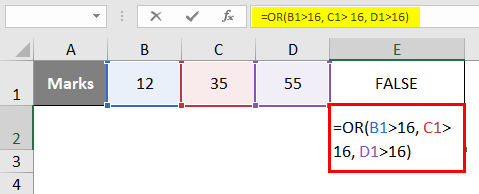
Press Enter key, and you can see the output as TRUE in cell E2 since C1 and D1 have values greater than 16. However, with E1, it is still FALSE since not all the conditions are satisfied.
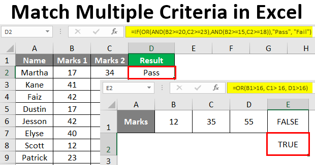
Example #2 – Complex Criteria in Combination with IF, AND/OR
Suppose we conduct two tests in a class of 10 students and have Marks in both tests for each student stored under column Marks 1 and Marks 2 respectively. We wanted to check whether the student has passed the exam or not. See the screenshot of the below data.
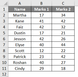
In order to check whether the student has passed the test or he failed, we can use a combination of IF statement with AND/OR operator to combine the multiple criteria.
Suppose we have two criteria’s under this example:
Criteria 1: Column B >= 20 and Column C >= 23
Criteria 2: Column B >= 15 and Column C >= 18
If either one of the criteria is fulfilled, the student will be declared as Pass; else, he/she will be declared as Fail. Let’s try to figure this tricky criterion out with IF, AND, OR.
Step 1: In cell D2, initiate the formula for IF Statement by typing “=IF(
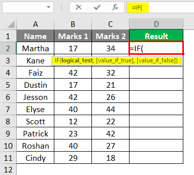
Step 2: Initiate an OR condition within the IF statement as shown below:
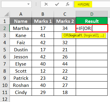
Step 3: Now, we need to add two AND conditions within this OR condition separated by a comma. Use (AND(B2>= 20, C2>=23), AND(B2>=15, C2>=18)) under OR condition within IF Statement and close the bracket for OR condition.
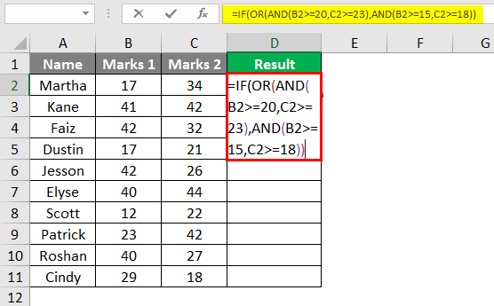
This condition will first check if Marks 1 and Marks 2 are greater than or equals to 20 and 23 respectively (first AND condition) OR if not, it will check whether the Marks 1 and Marks 2 are greater than or equals to 15 and 18 (second AND condition). If at least one of these two conditions is satisfied, the student will be considered as Pass; otherwise, the student will be considered a Fail.
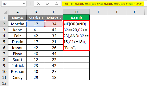
Step 4: Add the [value_if_true] as “Pass” under the formula in cell D2 to specify if at least one of the condition gets satisfied, a student is a pass.
Step 5: Add “Fail” as a value for [value_if_false] under the IF statement to complete the formula and close the brackets to complete it. Press Enter key to see the output in cell D2 whether the student named “Martha” has passed the exam or not.
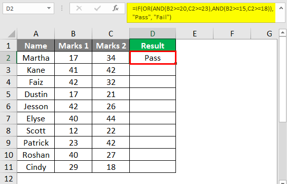
Step 6: Drag the formula across cells D2:D11 so that we will have a result value, either Pass or Fail, for all the students named in column A. You can select D2:D11 and then press Ctrl + D as a keyboard shortcut to be able to copy the formula across rows.
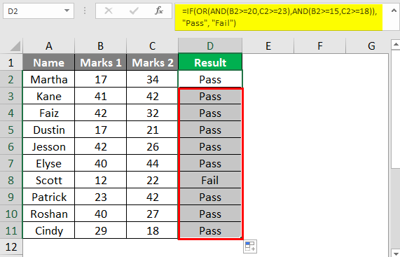
This is how we can match multiple criteria’s under Excel with the help of IF statement, AND & OR logical operators. This article ends here. Let’s wrap things up with some points to be remembered.
Things to Remember
- Logical operators such as AND, OR in combination with conditional statement IF are used to match multiple criteria under Excel.
- Microsoft Excel tests all the conditions under AND even if the previous condition is checked and appeared as FALSE. This is a bit unusual as in other programming languages if the previously checked condition is returned as FALSE under logical AND, the system stops checking other subsequent conditions.
- Logical AND returns TRUE if all the conditions inputted are satisfied. Otherwise, it returns as FALSE.
- Logical OR returns TRUE if at least one of the conditions is satisfied. If no other condition is satisfied, it returns as FALSE.
Recommended Article
This has been a guide to Excel Match Multiple Criteria. Here we discuss how to Match Multiple Criteria along with practical examples and a downloadable excel template. You can also go through our other suggested articles –
- INDEX MATCH Function in Excel
- Matching Columns in Excel
- VBA Match
- How to Match Data in Excel
We use the IF statement in Excel to test one condition and return one value if the condition is met and another if the condition is not met.
However, we use multiple or nested IF statements when evaluating numerous conditions in a specific order to return different results.
This tutorial shows four examples of using nested IF statements in Excel and gives five alternatives to using multiple IF statements in Excel.
General Syntax of Nested IF Statements (Multiple IF Statements)
The general syntax for nested IF statements is as follows:
=IF(Condition1, Value_if_true1, IF(Condition2, Value_if_true2, IF(Condition3, Value_if_true3, Value_if_false)))
This formula tests the first condition; if true, it returns the first value.
If the first condition is false, the formula moves to the second condition and returns the second value if it’s true.
Each subsequent IF function is incorporated into the value_if_false argument of the previous IF function.
This process continues until all conditions have been evaluated, and the formula returns the final value if none of the conditions is true.
The maximum number of nested IF statements allowed in Excel is 64.
Now, look at the following four examples of how to use nested IF statements in Excel.
Example #1: Use Multiple IF Statements to Assign Letter Grades Based on Numeric Scores
Let’s consider the following dataset showing some students’ scores on a Math test.

We want to use nested IF statements to assign student letter grades based on their scores.
We use the following steps:
- Select cell C2 and type in the below formula:
=IF(B2>=90,"A",IF(B2>=80,"B",IF(B2>=70,"C",IF(B2>=60,"D","F"))))

- Click Enter in the cell to get the result of the formula in the cell.
- Copy the formula for the rest of the cells in the column
The assigned letter grades appear in column C.

Explanation of the formula
=IF(B2>=90,”A”,IF(B2>=80,”B”,IF(B2>=70,”C”,IF(B2>=60,”D”,”F”))))
This formula evaluates the value in cell B2 and assigns an “A” if the value is 90 or greater, a “B” if the value is between 80 and 89, a “C” if the value is between 70 and 79, a “D” if the value is between 60 and 69, and an “F” if the value is less than 60.
Notice that it can be challenging to keep track of which parentheses go with which arguments in nested IF functions.
Therefore, as we enter the formula, Excel uses different colors for the parentheses at each level of the nested IF functions to make it easier to see which parts of the formula belong together.

Also read: How to use Excel If Statement with Multiple Conditions Range
Example #2: Use Multiple IF Statements to Calculate Commission Based on Sales Volume
Here’s the dataset showing the sales of specific salespeople in a particular month.

We want to use multiple IF statements to calculate the tiered commission for the salespeople based on their sales volume.
We proceed as follows:
- Select cell C2 and enter the following formula:
=IF(B2>=40000, B2*0.14,IF(B2>=20000,B2*0.12,IF(B2>=10000,B2*0.105,IF(B2>0,B2*0.08,0))))

- Press the Enter key to get the result of the formula.
- Double-click or drag the Fill Handle to copy the formula down the column.
The commission for each salesperson is displayed in column D.

Explanation of the formula
=IF(B2>=40000, B2*0.14,IF(B2>=20000,B2*0.12,IF(B2>=10000,B2*0.105,IF(B2>0,B2*0.08,0))))
This formula evaluates the value in cell B2 and then does the following:
- If the value in cell B2 is greater than or equal to 40,000, the figure is multiplied by 14% (0.14).
- If the figure in cell B2 is less than 40,000 but greater than or equal to 20,000, the value is multiplied by 12% (0.12).
- If the number in cell B2 is less than 20,000 but greater than or equal to 10,000, the figure is multiplied by 10.5% (0.105).
- If the value in cell B2 is less than 10,000 but greater than 0 (zero), the number is multiplied by 8% (0.08).
- If the value in cell B2 is 0 (zero), 0 (zero) is returned.
Example #3: Use Multiple IF Statements to Assign Sales Performance Rating Based On Sales Target Achievement
The following is a dataset showing regional sales data of a specific technology company in a particular year.

We want to use multiple IF statements to assign a sales performance rating to each region based on their sales target achievement.
We use the following steps:
- Select cell C2 and type in the below formula:
=IF(B2>500000, "Excellent", IF(B2>400000, "Good", IF(B2>275000, "Average", "Poor")))

- Click Enter on the Formula bar.
- Drag or double-click the Fill Handle to copy the formula down the column.
The performance ratings of the regions are shown in column C.

Explanation of the formula
=IF(B2>500000, “Excellent”, IF(B2>400000, “Good”, IF(B2>275000, “Average”, “Poor”)))
In this formula, if the sales target in cell B2 is greater than 500,000, the formula returns “Excellent.”
If it’s between 400,000 and 500,000, the formula returns “Good.”
If it’s between 275,000 and 400,000, the formula returns “Average.” And if it’s below 275,000, the formula returns “Poor.”
Example #4: Use Multiple IF Statements in Excel to Check For Errors and Return Error Messages
Suppose we have the following dataset of students’ English test scores. Some scores are less than 0 or greater than 100, and there are no scores in some cases.

We want to use nested IF statements to check for scores in column B and display error messages in column C if there are no scores or the scores are less than 0 or greater than 100.
If the score in column B is valid, we want the formula to return an empty string in column C.
Here are the steps to follow:
- Select cell C2 and enter the following formula:
=IF(OR(B2<0,B2>100),"Score out of range",IF(ISBLANK(B2),"Invalid score",""))

- Click Enter on the Formula bar.
- Drag the Fill Handle to copy the formula down the column.
The error messages are shown in column C.

Explanation of the formula
=IF(OR(B2<0,B2>100),”Score out of range”,IF(ISBLANK(B2),”Invalid score”,””))
This formula uses the OR function to check if the score in cell B2 is less than 0 or greater than 100, and if it is, it returns the error message “Score out of range.”
The formula also uses the ISBLANK function to check if cell B2 is blank, and if it is, it returns the error message “Invalid score.”
If there is no error, the formula returns an empty string, meaning no message is displayed in column B.
Alternatives to Using Multiple IF Statements in Excel
Formulas using nested IF statements can become difficult to read and manage if we have more than a few conditions to test.
In addition, if we exceed the maximum allowed limit of 64 nested IF statements, we will get an error message.
Fortunately, Excel offers alternative ways to use instead of nested IF functions, especially when we need to test more than a few conditions.
We present the alternative ways in this tutorial.
Alternative #1: Use the IFS Function
The IFS function tests whether one or more conditions are met and returns a value corresponding to the first TRUE condition.
Before the release of the IFS function in 2018 as part of the Excel 365 update, the only way to test multiple conditions and return a corresponding value in Excel was to use nested IF statements.
However, multiple IF statements have the downside of resulting in unwieldy formulas that are difficult to read and maintain.
In some situations, the IFS function is designed to replace the need for multiple IF functions.
The syntax of the IFS function is more straightforward and easier to read than nested IF statements, and it can handle up to 127 conditions.
Here’s an example:
Let’s consider the following dataset showing some students’ scores on a Math test.

We want to use the IFS function to assign letter grades to the students based on their scores.
We use the following steps:
- Select cell C2 and type in the below formula:
=IFS(B2>=90, "A", B2>=80, "B", B2>=70, "C", B2>=60, "D", B2<60, "F")

- Click Enter on the Formula bar.
- Drag or double-click the Fill Handle to copy the formula down the column.
The student’s letter grades are shown in column C.

Explanation of the formula
=IFS(B2>=90, “A”, B2>=80, “B”, B2>=70, “C”, B2>=60, “D”, B2<60, “F”)
This formula tests the score in cell B2 against each condition and returns the corresponding grade letter when the condition is true.
Limitation of IFS Function
The IFS function in Excel is designed to simplify complex nested IF statements.
However, there are situations where the IFS function may not be able to replace nested IF functions completely.
One such situation is when you must calculate or operate based on a condition or set of conditions.
While the IFS function can return a value or text string based on a condition, it cannot perform calculations or operations on that value like nested IF statements.
Another situation where the IFS function may be less useful is when you need to test for a range of conditions rather than just a specific set.
This is because the IFS function requires you to specify each condition and corresponding result separately, which can become cumbersome if you have many conditions to test—in contrast, nested IF statements allow you to test for a range of conditions using logical operators like AND and OR.
The IFS function is a powerful tool for simplifying complex logical tests in Excel.
However, there may be situations where nested IF statements are more appropriate for your needs.
We recommend that you consider both options and choose the one that best fits the specific requirements of your task.
Alternative #2: Use Nested IF Functions
We can use multiple IFS functions in a formula if we have more than one condition to test.
For example, let’s say we have the following dataset of student names and scores on a Physics test in columns A and B.

We want to assign a letter grade to each score and include a pass or fail designation based on whether the score is above or below 75.
Here are the steps to use:
- Select cell C2 and enter the following formula
=IFS(B2>=90,"A",B2>=80,"B",B2>=70,"C",B2>=60,"D",B2<60,"F")&" "&IFS(B2>=75,"Pass",B2<75,"Fail")

- Click Enter on the Formula bar.
- Drag or double-click the Fill Handle to copy the formula down the column.
The letter grade and designation of the student scores are displayed in column C.

Explanation of the formula
=IFS(B2>=90,”A”,B2>=80,”B”,B2>=70,”C”,B2>=60,”D”,B2<60,”F”)&” “&IFS(B2>=75,”Pass”,B2<75,”Fail”)
This formula uses the first IFS function to assign a letter grade based on the score in column A and the second IFS function to give a pass/fail designation based on the score in column A.
The two IFS functions are combined using the ampersand (&) operator to create a single text string that displays each score’s letter grade and pass/fail designation.
Alternative #3: Use the Combination of CHOOSE and XMATCH Functions
The CHOOSE function selects a value or action from a value list based on an index number.
The XMATCH function locates and returns the relative position of an item in an array. We can combine these functions in a formula instead of nested IF functions.
Here’s an example:
Suppose we have the following dataset showing some students’ scores and letter grades on a Biology test.

We want to use a formula combining the CHOOSE and XMATCH functions to assign corresponding grade points in column D to each letter grade.
We use the following steps:
- Select cell D2 and type in the below formula:
=CHOOSE(XMATCH(C2,{"F","E","D","C","B","A"},0),0,1,2,3,4,5)

- Click Enter on the Formula bar.
- Drag or double-click the Fill Handle to copy the formula down the column.
The grade points for each student are displayed in column D.

Explanation of the formula
=CHOOSE(XMATCH(C2,{“F”,”E”,”D”,”C”,”B”,”A”},0),0,1,2,3,4,5)
This formula applies the XMATCH function to find the position of the letter grade in the array {“F”,”E”,”D”,”C”,”B”,”A”}, and then uses the CHOOSE function to return the corresponding grade points.
Alternative #4: Use the VLOOKUP Function
The VLOOKUP function looks for a value in the leftmost column of a table and then returns a value in the same row from a specified column.
We can use the VLOOKUP function instead of nested IF functions in Excel.
The following is an example of using the VLOOKUP function instead of nested IF functions in Excel:
Suppose we have the following dataset showing some students’ scores and letter grades on a Biology test.

We want to use the VLOOKUP function to assign grade points to each student’s letter grade in column D.
We use the steps below:
- Create a table that lists the grades and their corresponding grade points in cell range F1:G7.

- In cell D2, type the following formula:
=VLOOKUP(C2,$F$2:$G$7,2,FALSE)
Note: Use the dollar signs to lock down the cell range F2:G7.

- Click Enter on the Formula bar.
- Drag or double-click the Fill Handle to copy the formula down the column.
The grade points for each student appear in column D.

Explanation of the formula
=VLOOKUP(C2,$F$2:$G$7,2,FALSE)
This formula uses the VLOOKUP function to look up the grade in cell C2 in the table in F2:G7 and return the corresponding grade point in the second column (i.e., column G).
The “FALSE” argument ensures that an exact match is required.
Alternative #5: Use a User-Defined Function
If you need to test more than a few conditions, consider creating a User Defined Function in VBA that can handle many conditions.
Here’s an example of using VBA code to replace nested IF functions in Excel:
Suppose we have the following dataset showing the sales of specific salespeople in a particular month.

We want to use a User Defined Function to calculate the commission for each salesperson based on the following rates:
- If the total sales are less than $10,000, the commission rate is 8%.
- If the total sales are equal to or greater than $10,000 but less than $20,000, the commission rate is 10.5%.
- If the total sales are equal to or greater than $20,000 but less than $40,000, the commission rate is 12%.
- If the sales are equal to or greater than $40,000, the commission rate is 14%
We use the following steps:
- Open the worksheet containing the sales dataset.
- Press Alt + F11 to launch the Visual Basic Editor.
- Click Insert on the menu bar and choose Module to insert a new module.

- Enter the following VBA code.
'Code developed by Steve Scott from https://spreadsheetplanet.com
Function COMMISSION(Sales As Double) As Double
    Const Rate1 = 0.08
    Const Rate2 = 0.105
    Const Rate3 = 0.12
    Const Rate4 = 0.14

'Calculate sales commissions

    Select Case Sales
        Case 0 To 9999.99: COMMISSION = Sales * Rate1
        Case 10000 To 19999.99: COMMISSION = Sales * Rate2
        Case 20000 To 39999.99: COMMISSION = Sales * Rate3
        Case Is >= 40000: COMMISSION = Sales * Rate4
    End Select

End Function
- Save the function procedure and the workbook as a Macro-Enabled Workbook.
- Press Alt + F11 to switch to the active worksheet with the sales dataset.
- Select cell C2 and enter the following formula:
=COMMISSION(B2)

- Click Enter on the Formula bar.
- Drag or double-click the Fill Handle to copy the formula down the column.
The commission for each salesperson is displayed in column C.

This VBA function takes the sales amount as an argument and returns the corresponding commission.
The User-Defined Function is a much simpler and easier-to-read solution than using nested IF functions.
This tutorial showed four examples of using nested IF statements in Excel and gave five alternatives to using multiple IF statements in Excel. We hope you found the tutorial helpful.
Other Excel tutorials you may find useful:
- Excel Logical Test Using Multiple If Statements in Excel [AND/OR]
- How to Compare Two Columns in Excel (using VLOOKUP & IF)
- Using IF Function with Dates in Excel (Easy Examples)
- COUNTIF Greater Than Zero in Excel
- BETWEEN Formula in Excel (Using IF Function) – Examples
- Count Cells Less than a Value in Excel (COUNTIF Less)
Sometimes we need to make small amendments to formulas to make them effective.
Just like that, SUMIF OR. It’s an advanced formula that helps you to increase the flexibility of SUMIF. Yes, you can also do SUMIFS as well. But before we use it let me tell you one thing about SUMIF.
In SUMIF, you can only use one criterion and in SUMIFS, you can use more than one criterion to get a sum.
Just a thing like this. Let’s say, in SUMIFS, if you specify two different criteria, it will sum only those cells which meet both of the criteria.
Because it works with AND logic, all the criteria should meet to get a cell included. When you combine OR logic with SUMIF/SUMIFS you can sum values using two different criteria at the same time.
Without any further ado let’s learn this amazing formula.
Do We Really Need OR Logic? Any Example?
Let me show you an example where we need to add an OR logic in SUMIFS or SUMIF.
Take a look at below data table where you have a list of products with their quantity and the current status of the shipment.

In this data, you have two types of products (Faulty and Damaged) that you need to return to our vendor.
But before that, you want to calculate the total quantity of both types of products. If you go with the normal method, you have to apply SUMIF twice to get this total.
But if you use an OR condition in SUMIF then you can get the total of both of the products with just one formula.
OK, Let’s Apply OR with SUMIFS
Before we start, please download this sample file from here to follow along.
In any other cell in your worksheet where you want to calculate the total, insert the below formula and hit enter.
=SUM(SUMIFS(C2:C21,B2:B21,{"Damage","Faulty"}))
In the above formula, you have used SUMIFS but if you want to use SUMIF you can insert the below formula in the cell.
=SUM(SUMIF(B2:B21,{"Damage","Faulty"},C2:C21))By using both of the above formulas you will get 540 in the result. To cross-verify, just check the total manually.

How this formula Works
As I said, the SUMIFS function uses AND logic to sum values. But, the formula which you have used above includes an OR logic in it.
To understand this formula you have to split it into three different parts.

- The first thing is to understand that, you have used two different criteria in this formula by using the array concept. Learn more about the array from here.
- The second thing is when you specify two different values using an array, SUMIFS has to look for both of the values separately.
- The third thing is even after using an array formula, SUMIFS is not able to return the sum of both of the values in a single cell. So, that’s why you have to enclose it with the SUM function.
With the above concept, you are able to get a total for both types of products in a single cell.
It will work the same with SUMIF and SUMIFS.
And, you can also further expand your formula by specifying the product name in the second criteria in SUMIFS to get the total for a single product.
sample-file
Using Dynamic Criteria Range
In the comment section, Shay asked me about using a cell reference to add multiple criteria instead of inserting them directly into the formula.
Well, that’s a super valid question and you can do this by using a dynamic named range instead of hardcore values.
And for this, you need to do just two little amendments to your formula.
- The first is that instead of using curly brackets you need to use a named range (the best way is to use a table) of your value.
- And after that, you need to enter this formula by using Ctrl + Shift + Enter as a proper array formula.
So, now your formula will be:

Let me take you to next level of this formula. Just look at the below data table.

In this table, you have two different columns with two different kinds of statuses. Now, from this data table, you need to sum the quantity where the product is damaged return status is “No”.
That means only those Damage and Faulty products which are not been returned yet. And, the formula for this will be.
=SUM(SUMIFS(D2:D21,B2:B21,{"Damage","Faulty"},C2:C21,"No"))
sample-file
Conclusion
The best part about using the OR technique is you can add as many criteria to it. If you want to use only OR logic then it’s fine to use SUMIF. And if you want to create an OR condition and AND condition in a single formula then you can use SUMIFS for that.
You know, this is one of my favorite formula tips and I hope you found it useful.
Now tell me one thing. Have you ever used this kind of formula before? Share your views with me in the comment section, I’d love to hear from you, and please don’t forget to share this tip with your friends.