
Содержание
- SIGN Function
- Summary
- Purpose
- Return value
- Arguments
- Syntax
- Usage notes
- Examples
- Notes
- Dave Bruns
- IS functions
- Description
- Syntax
- Remarks
- Examples
- Example 1
- IS functions
- Description
- Syntax
- Remarks
- Examples
- Example 1
- IF Function
- Related functions
- Summary
- Purpose
- Return value
- Arguments
- Syntax
- Usage notes
- Syntax
- Logical tests
- IF cell contains specific text
- Logical functions in Excel with the examples of their use
- Logical functions in Excel and examples of solving the problems
- The use of logic functions in Excel:
- The function IF can be used as arguments to the text values
- The statistical and logical functions in Excel
SIGN Function

Summary
The Excel SIGN function returns the sign of a number as +1, -1 or 0. If number is positive, SIGN returns 1. If number is negative, sign returns -1. If number is zero, SIGN returns 0.
Purpose
Return value
Arguments
- number — The number to get the sign of.
Syntax
Usage notes
The SIGN function returns the sign of a number as +1, -1 or 0. If number is positive, SIGN returns 1. If number is negative, sign returns -1. If number is zero, SIGN returns 0.
The SIGN function takes one argument, number, which must be a numeric value. If number is not numeric, SIGN returns a #VALUE! error.
Examples
SIGN can be used to change negative numbers into positive values like this. For example, with -3 in cell A1, the formula below returns 3:
The formula above has no effect on positive numbers, since SIGN will return 1. However, the ABS function provides a simpler solution:
Notes
- If number is in the range (-∞,0) SIGN(number) will return -1.
- If number is equal to 0 SIGN(number) will return 0.
- If number is in the range (0,∞)(number) SIGN will return 1.
Dave Bruns
Hi — I’m Dave Bruns, and I run Exceljet with my wife, Lisa. Our goal is to help you work faster in Excel. We create short videos, and clear examples of formulas, functions, pivot tables, conditional formatting, and charts.
Источник
IS functions
Description
Each of these functions, referred to collectively as the IS functions, checks the specified value and returns TRUE or FALSE depending on the outcome. For example, the ISBLANK function returns the logical value TRUE if the value argument is a reference to an empty cell; otherwise it returns FALSE.
You can use an IS function to get information about a value before performing a calculation or other action with it. For example, you can use the ISERROR function in conjunction with the IF function to perform a different action if an error occurs:
= IF( ISERROR(A1), «An error occurred.», A1 * 2)
This formula checks to see if an error condition exists in A1. If so, the IF function returns the message «An error occurred.» If no error exists, the IF function performs the calculation A1*2.
Syntax
The IS function syntax has the following argument:
value Required. The value that you want tested. The value argument can be a blank (empty cell), error, logical value, text, number, or reference value, or a name referring to any of these.
Returns TRUE if
Value refers to an empty cell.
Value refers to any error value except #N/A.
Value refers to any error value (#N/A, #VALUE!, #REF!, #DIV/0!, #NUM!, #NAME?, or #NULL!).
Value refers to a logical value.
Value refers to the #N/A (value not available) error value.
Value refers to any item that is not text. (Note that this function returns TRUE if the value refers to a blank cell.)
Value refers to a number.
Value refers to a reference.
Value refers to text.
The value arguments of the IS functions are not converted. Any numeric values that are enclosed in double quotation marks are treated as text. For example, in most other functions where a number is required, the text value «19» is converted to the number 19. However, in the formula ISNUMBER( «19»), «19» is not converted from a text value to a number value, and the ISNUMBER function returns FALSE.
The IS functions are useful in formulas for testing the outcome of a calculation. When combined with the IF function, these functions provide a method for locating errors in formulas (see the following examples).
Examples
Example 1
Copy the example data in the following table, and paste it in cell A1 of a new Excel worksheet. For formulas to show results, select them, press F2, and then press Enter. If you need to, you can adjust the column widths to see all the data.
Источник
IF Function
Summary
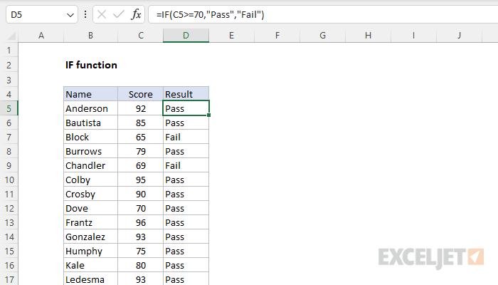
The Excel IF function runs a logical test and returns one value for a TRUE result, and another for a FALSE result. For example, to «pass» scores above 70: =IF(A1>70,»Pass»,»Fail»). More than one condition can be tested by nesting IF functions. The IF function can be combined with logical functions like AND and OR to extend the logical test.
Purpose
Return value
Arguments
- logical_test — A value or logical expression that can be evaluated as TRUE or FALSE.
- value_if_true — [optional] The value to return when logical_test evaluates to TRUE.
- value_if_false — [optional] The value to return when logical_test evaluates to FALSE.
Syntax
Usage notes
The IF function runs a logical test and returns one value for a TRUE result, and another value for a FALSE result. The result from IF can be a value, a cell reference, or even another formula. By combining the IF function with other logical functions like AND and OR, you can test more than one condition at a time.
Syntax
The generic syntax for the IF function looks like this:
The first argument, logical_test, is typically an expression that returns either TRUE or FALSE. The second argument, value_if_true, is the value to return when logical_test is TRUE. The last argument, value_if_false, is the value to return when logical_test is FALSE. Both value_if_true and value_if_false are optional, but you must provide one or the other. For example, if cell A1 contains 80, then:
Notice that text values like «OK», «Yes», «No», etc. must be enclosed in double quotes («»). However, numeric values should not be enclosed in quotes.
Logical tests
The IF function supports logical operators (>, ,=) when creating logical tests. Most commonly, the logical_test in IF is a complete logical expression that will evaluate to TRUE or FALSE. The table below shows some common examples:
| Goal | Logical test | ||||||||||||||||||||||||||||||||
|---|---|---|---|---|---|---|---|---|---|---|---|---|---|---|---|---|---|---|---|---|---|---|---|---|---|---|---|---|---|---|---|---|---|
| If A1 is greater than 75 | A1>75 | ||||||||||||||||||||||||||||||||
| If A1 equals 100 | A1=100 | ||||||||||||||||||||||||||||||||
| If A1 is less than or equal to 100 | A1 «red» | ||||||||||||||||||||||||||||||||
| If A1 is less than B1 | A1 «» | ||||||||||||||||||||||||||||||||
| If A1 is less than current date | A1 and less than 10, return «OK». Otherwise, return nothing («»).
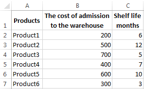
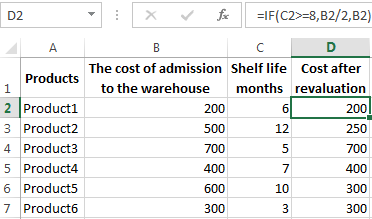
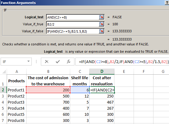
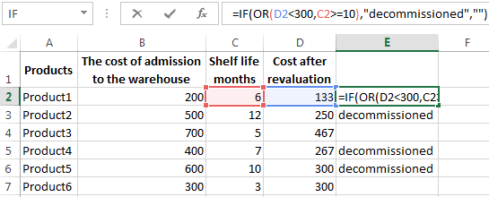
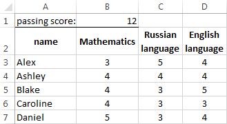
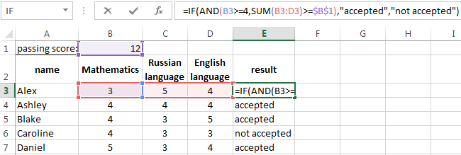
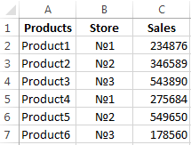
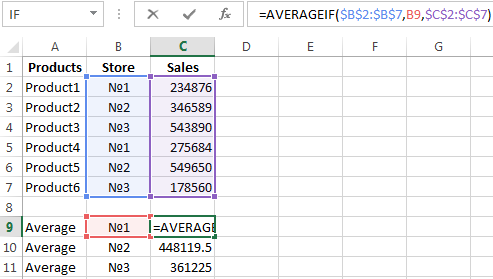
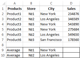
To return B1+10 when A1 is «red» or «blue» you can use the OR function like this: Translation: if A1 is red or blue, return B1+10, otherwise return B1. Translation: if A1 is NOT red, return B1+10, otherwise return B1. IF cell contains specific textBecause the IF function does not support wildcards, it is not obvious how to configure IF to check for a specific substring in a cell. A common approach is to combine the ISNUMBER function and the SEARCH function to create a logical test like this: For example, to check for the substring «xyz» in cell A1, you can use a formula like this: Источник Logical functions in Excel with the examples of their useLogic Functions in Excel check the data and return the result «TRUE» if the condition is true, and «FALSE» if not. Consider the syntax of logic functions and examples of their application in the process of working with the Excel program. Logical functions in Excel and examples of solving the problemsObjective 1. It is necessary to overestimate the trade balances. If he product is kept in stock for more than 8 months we should reduce its price 2 times. We form a table with initial parameters: To solve the problem, use the logical IF function. The formula will have a look like this: =IF(C2>=8;B2/2;B2) Logical expression «C2>=8» is constructed using relational operators «>» and «=». The result of his calculations is a logical value of «TRUE» or «FALSE». In the first case, the function returns the value «B2/2». In the second it’s «B2». Let’s complicate the task — to employ the logic function И. Now we have such a condition: if the product is stored for more than 8 months, the price is reduced 2 times. If it’s more than 5 months, but less than 8, it’s 1.5 times. The formula takes the following form: =8),B2/2,IF(AND(C2>=5),B2/1.5,B2))’ > The use of logic functions in Excel:
The function IF can be used as arguments to the text valuesFor the solution use logic functions IF and OR: Condition recorded using a logical OR operation, stands as follows: goods are deducted if the number in cell D2 = 10. In terms of non-compliance with the conditions, IF function returns to an empty cell. As arguments, you can use other functions. These are mathematical, for example. Objective 3. Students before entering the gymnasium pass math, English and Russian. Passing Score is 12. You should get at least 4 points in mathematics for admission. Create report on the receipt. We set up a table with the source data: It is necessary to compare the total number of points with a passing grade. And check that math score was not lower than «4». In the «result» column put «accepted» or «not accepted». There’s such a formula: Logical operator «AND» causes the function to check the validity of the two conditions. The mathematical function «SUM» is used to calculate the final score. The function IF allows us to solve many problems; it is therefore used more often. The statistical and logical functions in ExcelTask 1. Analyze the cost of cash balances after the devaluation. If the price of the product after reassessment is below average values, we should write off the product from the warehouse. Working with the table in the previous section: To solve the problem use the formula of such a form: Task 2. Find the average sales in stores. We set up a table with the source data: You need to find the arithmetic meaning for the cells, which value corresponds to a predetermined condition. That is to combine logical and statistical solution. Below a table with a condition there’s the table to display the results. We solve the problem with a single function: The first argument $B$2:$B$7 is a range of cells for testing. The second argument B9 is a condition. The third argument the $C$2:$C$7 is an averaging range; the numerical values, which are taken to calculate the arithmetic mean. AVERAGEIF function compares the value of B9 cells (№1) with values in the range B2: B7. That is the number of stores in the sales table. For matching the data considers the arithmetic mean of using numbers in the range C2: C7. Task 3. Find the average sales in the store №1 New York and №2 Los Angeles. Modify the table from the previous example: It is necessary to fulfill two conditions — use the function of the form: The function AVERAGEIFS allows you to use more than one condition. The first argument $D$2:$D$7 is an averaging ranges (where are the numbers to find the arithmetic mean). The second argument $B$2:$B$7 is a range to test the first condition. The third argument B9 is the first condition. The fourth and fifth arguments are the ranges for checking the second condition respectively. The function takes into account only the values that meet all these criteria. Источник Adblock |
This post will guide you on how to show only positive values in Excel. There are several ways to accomplish this, including formatting cells, using conditional formatting, and using VBA code.
We will discuss each method in detail and provide step-by-step instructions on how to implement them.
Table of Contents
- 1. Video: Show Only Positive Values
- 2. Show Only Positive Numbers in a Range with Format Cells
- 3. Show Only Positive Numbers in a Range with Conditional Formatting
- 4. Show Only Positive Numbers in a Range with VBA Code
- 5. Show Only Positive Values after Calculating
- 6. Related Functions
In this video, we will explore various methods, such as formatting cells, using conditional formatting, and VBA code, to show only positive values in Excel.
2. Show Only Positive Numbers in a Range with Format Cells
To only display positive numbers in a range using the Format Cells feature in Microsoft Excel, follow these steps:
Step1: Select one range that you want to format.
Step2: Right-click and select “Format Cells” from the context menu.
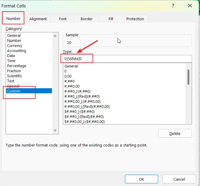
Step3: In the Format Cells dialog box, select the “Number” tab. Select “Custom” from the Category list. In the “Type” field, enter the following format code: 0;[White0 , Click “OK” to apply the formatting.
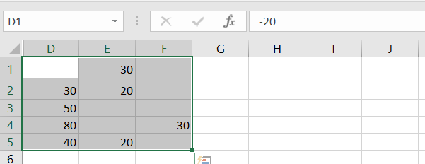
Step3: only positive numbers in the selected range will be displayed.
3. Show Only Positive Numbers in a Range with Conditional Formatting
If you only want to highlight or format positive numbers in a range, you can also use the Conditional Formatting feature in Microsoft Excel, just do the following steps:
Step1: Select one range that want to format.
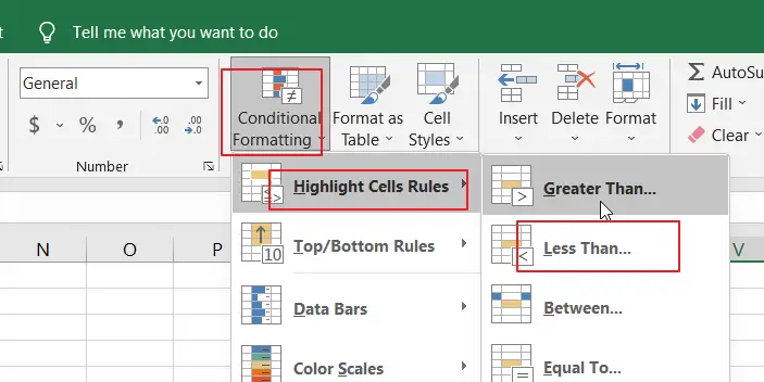
Step2: Click on the “Conditional Formatting” button in the “Home” tab of the ribbon. Select “Highlight Cell Rules” and then “Less Than” from the dropdown menu.
Step3: In the “Less Than” dialog box, enter “0” in the “Value” field. Choose “Custom Format…”, then set the font color as white.
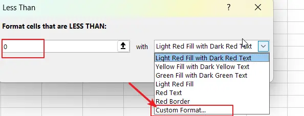
Step3: Click “OK” to apply the formatting.
This will only show all cells in the selected range that contain a value greater than zero.
4. Show Only Positive Numbers in a Range with VBA Code
If you want to show positive numbers in a range using VBA code, you can use a loop to iterate through each cell in the range and check if the value is greater than zero. If the value is positive, you can keep it in the cell. Otherwise, you can set font color as white.
Just refer to the following steps:
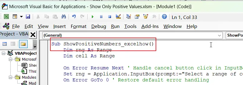
Step1: Press Alt + F11 on your keyboard. This will open the Visual Basic Editor.
![]()
Step2: Go to the menu bar at the top of the Visual Basic Editor and click on Insert -> Module. This will create a new module in the project.
![]()
Step3: Copy the following VBA code you want to run and paste it into the module. Save the VBA code and close the Visual Basic Editor.
Sub ShowPositiveNumbers_excelhow()
    Dim rng As Range
    Dim cell As Range

    On Error Resume Next ' Handle cancel button click in InputBox
    Set rng = Application.InputBox(prompt:="Select a range of cells", Type:=8)
    On Error GoTo 0 ' Restore default error handling

    If Not rng Is Nothing Then ' Check if a range was selected
        For Each cell In rng
            If cell.Value < 0 Then
                cell.Font.Color = RGB(255, 255, 255)
            End If
        Next cell
    End If
End Sub
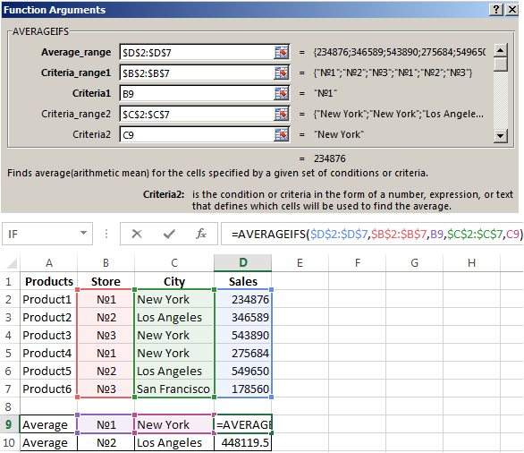
Step4: Press Alt + F8 to open the Macros dialog box. Select the macro you want to run and click on the Run button.
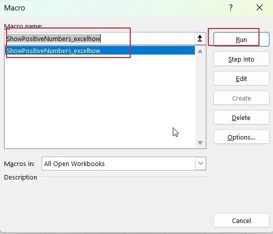
Step5: select a range of cells that you want to filter all positive values.
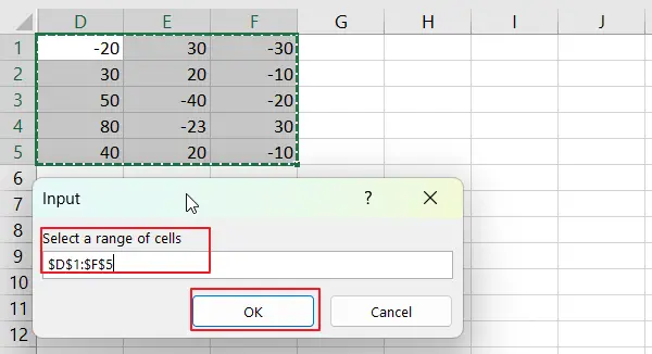
Step5: You can see that only positive values are shown in your selected range of cells.
5. Show Only Positive Values after Calculating
Assuming that you have a list of data, and you want to sum the range of cells A1:C5 and if the summation result is greater than 0 or is a positive number, then display this result. Otherwise, display as a blank cell.
You can create a formula based on the IF function, and the SUM function to sum all values in the range A1:C5 and just show only positive values. Like this:
=IF(SUM(A1:C1)<0, "",SUM(A1:C1))Type this formula into the formula box of the cell D1, then drag AutoFill Handler over other cells to apply this formula.
You will see that the returned results of this formula only show positive values.
- Excel SUM function
The Excel SUM function will adds all numbers in a range of cells and returns the sum of these values. You can add individual values, cell references or ranges in excel.The syntax of the SUM function is as below:= SUM(number1,[number2],…)… - Excel IF function
The Excel IF function perform a logical test to return one value if the condition is TRUE and return another value if the condition is FALSE. The IF function is a build-in function in Microsoft Excel and it is categorized as a Logical Function.The syntax of the IF function is as below:= IF (condition, [true_value], [false_value])….
METHOD 1. Convert negative numbers to positive using VBA with the ABS Function
VBA
Sub Convert_negative_numbers_to_positive()
Dim ws As Worksheet
Set ws = Worksheets(«Analysis»)
ws.Range(«C5») = Abs(ws.Range(«B5»))
ws.Range(«C6») = Abs(ws.Range(«B6»))
ws.Range(«C7») = Abs(ws.Range(«B7»))
End Sub
OBJECTS
Worksheets: The Worksheets object represents all of the worksheets in a workbook, excluding chart sheets.
Range: The Range object is a representation of a single cell or a range of cells in a worksheet.
PREREQUISITES
Worksheet Name: Have a worksheet named Analysis.
Numbers: If using the same VBA code you need to ensure that the numbers that you want to convert to positive are captured in range («B5:B7»).
ADJUSTABLE PARAMETERS
Output Range: Select the output range by changing the cell references («C5»), («C6») and («C7») in the VBA code to any cell in the worksheet, that doesn’t conflict with the formula.
Numbers: Select the numbers which you want to convert to positive by changing range («B5:B7»), that doesn’t conflict with the formula.
ADDITIONAL NOTES
Note 1: The application of this VBA code is practical in a scenario where there are only limited number of values that you want to convert to positive numbers. You don’t want to be typing the same code for each number that you want to convert. Therefore, in a scenario where you want to convert a large range of numbers you can apply the For Loop, which is shown in the following VBA method (Method 2).
METHOD 2. Convert negative numbers to positive using VBA with the ABS Function and For Loop
VBA
Sub Convert_negative_numbers_to_positive()
Dim ws As Worksheet
Set ws = Worksheets(«Analysis»)
For x = 5 To 7
ws.Range(«C» & x) = Abs(ws.Range(«B» & x))
Next x
End Sub
OBJECTS
Worksheets: The Worksheets object represents all of the worksheets in a workbook, excluding chart sheets.
Range: The Range object is a representation of a single cell or a range of cells in a worksheet.
PREREQUISITES
Worksheet Name: Have a worksheet named Analysis.
Numbers: If using the exact same VBA code you need to ensure that the numbers that you want to convert to positive are captured in range («B5:B7»).
ADJUSTABLE PARAMETERS
Output Range: In this example we are using the x value to drive the output row number, which has to match the row which captures the number that you want to convert. To change the column in which to return the converted value you need to change the column C reference in the VBA code.
Numbers: In this example we are using the x value to drive the row number of the values which you want to convert to positive. To change the column in which the numbers that you want to convert are captured you will need to change the column B reference in the VBA code.
METHOD 3. Convert negative numbers to positive using VBA with the IF Function
VBA
Sub Convert_negative_numbers_to_positive()
Dim ws As Worksheet
Set ws = Worksheets(«Analysis»)
If ws.Range(«B5») < 0 Then
ws.Range(«C5») = ws.Range(«B5») * -1
Else
ws.Range(«C5») = ws.Range(«B5»)
End If
If ws.Range(«B6») < 0 Then
ws.Range(«C6») = ws.Range(«B6») * -1
Else
ws.Range(«C6») = ws.Range(«B6»)
End If
If ws.Range(«B7») < 0 Then
ws.Range(«C7») = ws.Range(«B7») * -1
Else
ws.Range(«C7») = ws.Range(«B7»)
End If
End Sub
OBJECTS
Worksheets: The Worksheets object represents all of the worksheets in a workbook, excluding chart sheets.
Range: The Range object is a representation of a single cell or a range of cells in a worksheet.
PREREQUISITES
Worksheet Name: Have a worksheet named Analysis.
Numbers: If using the exact same VBA code you need to ensure that the numbers that you want to convert to positive are captured in range («B5:B7»).
ADJUSTABLE PARAMETERS
Output Range: Select the output range by changing the cell references («C5»), («C6») and («C7») in the VBA code to any cell in the worksheet, that doesn’t conflict with the formula.
Numbers: Select the numbers which you want to convert to positive by changing range («B5:B7»).
ADDITIONAL NOTES
Note 1: The application of this VBA code is practical in a scenario where there are only limited number of values that you want to convert to positive numbers. You don’t want to be retyping the same code for each number that you want to convert. Therefore, in a scenario where you want to convert a large range of numbers you can apply the For Loop, which is shown in the following VBA method (Method 4).
METHOD 4. Convert negative numbers to positive using VBA with the IF Function and For Loop
VBA
Sub Convert_negative_numbers_to_positive()
Dim ws As Worksheet
Set ws = Worksheets(«Analysis»)
For x = 5 To 7
If ws.Range(«B» & x) < 0 Then
ws.Range(«C» & x) = ws.Range(«B» & x) * -1
Else
ws.Range(«C» & x) = ws.Range(«B» & x)
End If
Next x
End Sub
OBJECTS
Worksheets: The Worksheets object represents all of the worksheets in a workbook, excluding chart sheets.
Range: The Range object is a representation of a single cell or a range of cells in a worksheet.
PREREQUISITES
Worksheet Name: Have a worksheet named Analysis.
Numbers: If using the exact same VBA code you need to ensure that the numbers that you want to convert to positive are captured in range («B5:B7»).
ADJUSTABLE PARAMETERS
Output Range: In this example we are using the x value to drive the output row number, which has to match the row which captures the number that you want to convert. To change the column in which to return the converted value you need to change the column C reference in the VBA code.
Numbers: In this example we are using the x value to drive the row number of the values which you want to convert to positive. To change the column in which the numbers that you want to convert are captured you will need to change the column B reference in the VBA code.
METHOD 5. Convert negative numbers to positive using VBA in selected range
VBA
Sub Convert_negative_numbers_to_positive()
Dim conv As Range
For Each conv In Selection
If conv.Value < 0 Then
conv.Offset(0, 1) = -conv.Value
Else
conv.Offset(0, 1) = conv.Value
End If
Next conv
End Sub
PREREQUISITES
Selection: This example converts all of the selected values to positive, therefore, before running this VBA code you need to select a cell or a range of cells that you want to convert from negative to positive numbers.
ADDITIONAL NOTES
Note 1: This VBA code converts the negative numbers to positive and returns the values in the adjacent column.
METHOD 6. Convert negative numbers to positive using VBA in selected range
VBA
Sub Convert_negative_numbers_to_positive()
Dim conv As Range
For Each conv In Selection
If conv.Value < 0 Then
conv.Value = -conv.Value
End If
Next conv
End Sub
PREREQUISITES
Selection: This example converts all of the selected values to positive, therefore, before running this VBA code you need to select a cell or a range of cells that you want to convert from negative to positive numbers.
ADDITIONAL NOTES
Note 1: This VBA code converts the negative numbers to positive and returns the values in the selected range, therefore, replacing the numbers that you have selected.
Explanation about the formulas used to convert negative numbers to positive
EXPLANATION
DESCRIPTION
This tutorial explains how to convert negative numbers to positive numbers by applying Excel and VBA methods.
Excel Methods: This tutorial provides two Excel methods that can be applied to convert negative numbers to positive. The first method uses the Excel ABS Function, which returns an absolute number.
The second method uses the Excel IF function to test if the selected number is negative and if so the formula will multiply the number by -1, converting it to a positive number. If the test is FALSE, the formula will return the same number (which will be positive).
VBA Methods: This tutorial provides six VBA methods that can be applied to convert negative numbers to positive. The first two methods use the Abs function, which returns an absolute number. The first method is practical if there are only a limited number of values to convert (e.g. two or three), given we have applied the same code against each of the numbers that we want to convert. However, if you want to convert a large amount of numbers in a range, we can use the For Loop, combined with the Abs function, which is shown in VBA Method 2.
The third and fourth methods use the Excel IF function to test if the selected number is negative and if so the formula will multiply the number by -1, converting it to a positive number. If the test is FALSE, the formula will return the same number. As per above, the third method is practical if there are only a limited number of values to convert (e.g. two or three), given we have applied the same code against each of the numbers that we want to convert. However, if you want to convert a large amount of numbers in a range, we can use the For Loop, combined with the IF function, which is shown in VBA Method 4.
The fifth and sixth methods convert only the selected numbers. The difference between the fifth and the sixth method is that the fifth method returns the converted numbers in the adjacent column, whilst the sixth method replaces the selected values.
FORMULA (using ABS Function)
=ABS(number)
FORMULA (using IF Function)
=IF(number<0, number*-1, number)
ARGUMENTS
number: A numeric value to be converted from into a positive number.
The SIGN function returns the sign of a number as +1, -1 or 0. If number is positive, SIGN returns 1. If number is negative, sign returns -1. If number is zero, SIGN returns 0.
The SIGN function takes one argument, number, which must be a numeric value. If number is not numeric, SIGN returns a #VALUE! error.
Examples
=SIGN(5) // returns 1
=SIGN(-3) // returns -1
=SIGN(0) // returns 0
SIGN can be used to change negative numbers into positive values like this. For example, with -3 in cell A1, the formula below returns 3:
=A1*SIGN(A1)
=-3*-1
=3
The formula above has no effect on positive numbers, since SIGN will return 1. However, the ABS function provides a simpler solution:
=ABS(A1) // absolute value of A1
Notes
- If number is in the range (-∞,0) SIGN(number) will return -1.
- If number is equal to 0 SIGN(number) will return 0.
- If number is in the range (0,∞)(number) SIGN will return 1.
Multiply with Minus One to Convert a Positive Number So you can use the same method in excel to convert a negative number into a positive. All you have to do just multiply a negative value with -1 and it will return the positive number instead of the negative.
Contents
- 1 How do I make a number always positive in Excel?
- 2 How do you make a number positive?
- 3 How do I make all numbers positive?
- 4 How do I make a number absolute in Excel?
- 5 How do I change numbers to negative in Excel?
- 6 How do you make an equation positive?
- 7 How do you make negative numbers red in Excel?
- 8 How do I use F4 in Excel?
- 9 How do you make an absolute value in Excel without F4?
- 10 What is absolute in Excel?
- 11 How do you turn a negative into a positive?
- 12 What is as a positive number?
- 13 How do you add negative and positive variables?
- 14 Is it possible to have a negative variable?
- 15 What To Do If A is negative in standard form?
- 16 How do I highlight positive and negative numbers in Excel?
- 17 How do you make a positive percentage Green in Excel?
- 18 How do I make an Excel cell Red or Green?
ABS Formula In Excel
In Excel, you compute the absolute value using the formula function ABS. With the formula =ABS(-5), Excel converts the negative to positive and gives the result 5. You can wrap a larger computation in the ABS function to make the result always positive.
How do you make a number positive?
Multiply with Minus One to Convert a Positive Number
All you have to do just multiply a negative value with -1 and it will return the positive number instead of the negative.
How do I make all numbers positive?
Steps to Make All Numbers Positive in Excel
- Next to the data that you want to make positive, type =ABS(cell reference) like this:
- Once you enter that function simply copy it down by selecting cell B1 and double-clicking the bottom right corner of the cell.
How do I make a number absolute in Excel?
Create an Absolute Reference
Select a cell, and then type an arithmetic operator (+, -, *, or /). Select another cell, and then press the F4 key to make that cell reference absolute. You can continue to press F4 to have Excel cycle through the different reference types.
How do I change numbers to negative in Excel?
Change positive numbers to negative or vice versa with Kutools for Excel
- Select the range you want to change.
- Click Kutools > Content > Change Sign of Values, see screenshot:
- And in the Change Sign of Values dialog box, select Change all positive values to negative option.
- Then click OK or Apply.
How do you make an equation positive?
You just have to simply multiply by −1. For example if you have a number −a then multiply by −1 to get −a×−1=a. If the number is positive then multiply by 1.
How do you make negative numbers red in Excel?
Here are the steps to do this:
- Go to Home → Conditional Formatting → Highlight Cell Rules → Less Than.
- Select the cells in which you want to highlight the negative numbers in red.
- In the Less Than dialog box, specify the value below which the formatting should be applied.
- Click OK.
How do I use F4 in Excel?
How to use F4 in Excel. Using the F4 key in Excel is quite easy. Think of a situation where you have been working on an Excel worksheet and you want to repeat the last action multiple times. All you need to do is press and hold Fn and then press and release the F4 key.
How do you make an absolute value in Excel without F4?
This is easily fixed! Just hold down the Fn key before you press F4 and it’ll work. Now, you’re ready to use absolute references in your formulas.
What is absolute in Excel?
In an Excel spreadsheet, a cell reference specifies an individual cell or a range of cells that is to be included in a formula.In contrast, the definition of absolute cell reference is one that does not change when it’s moved, copied or filled.
How do you turn a negative into a positive?
Think of anything positive to replace your negative thoughts. Instead of getting down about something, find something to be happy about and use this optimistic thought to replace your pessimistic thoughts. Practicing this over time, your mind will begin to focus on the good rather than the bad.
What is as a positive number?
A positive number is any number that represents more than zero of anything. Positive numbers include the natural, or counting numbers like 1,2,3,4,5, as well as fractions like 3/5 or 232/345, and decimals like 44.3.Zero is neither negative, nor positive.
How do you add negative and positive variables?
Adding Positive and Negative Numbers
- Rule 1: Adding positive numbers to positive numbers—it’s just normal addition.
- Rule 2: Adding positive numbers to negative numbers—count forward the amount you’re adding.
- Rule 3: Adding negative numbers to positive numbers—count backwards, as if you were subtracting.
Is it possible to have a negative variable?
Variables can be negative or positive in nature. Learn to manipulate variables in a variety of ways if you take a high school or college algebra or calculus course.A negative variable times a positive variable will produce a negative product. For example, -x * y = -xy.
What To Do If A is negative in standard form?
In standard form, A must always be positive, so if it is negative, divide each term by -1.
How do I highlight positive and negative numbers in Excel?
Select the data, then go to, Home | Conditional Formatting | New Rule | use a formula to determine which cells to format. Then select the format you wish to apply. click OK.
How do you make a positive percentage Green in Excel?
How to Format Percent Change in Excel
- Select the cell or cells with the percent change number.
- From the drop down select More Number Formats… at the bottom of the list.
- From the custom formats you paste in the values below in the Type box.
- Your custom formatting will look like this in your Excel Sheet.
How do I make an Excel cell Red or Green?
Re: RE: How do I make excel change the colour of a cell depending on a different cells date?
- Select cell A2.
- click Conditional Formatting on the Home ribbon.
- click New Rule.
- click Use a formula to determine which cells to format.
- click into the formula box and enter the formula.
- click the Format button and select a red color.
And you will be amazed that I have got seven different ways you can use to deal with negative numbers. Last week, I got an email from one of my subscribers with a question.
Hey Puneet, how many methods do we have to convert a negative number into a positive one?
You know, the thing for which he asked is a common kind of task. I am sure, this often happens to you, when you get some negative numeric values, and after that, you convert them into positive ones.
There is no #rocketscience in this. But have you ever checked how my different methods you have to do this? Well, I am always curious to know about different methods to do a task in Excel.
So this time I grabbed a paper and listed all the methods which I can use to convert a negative number into a positive. So today in this post, I’d like to share all those methods with you.
Let’s get started.
1. Multiply with Minus One to Convert a Positive Number
Unlike me, if you are good at maths, I am sure you know that when you multiply two minus signs with each other, the result is always positive. So you can use the same method in excel to convert a negative number into a positive.
All you have to do is just multiply a negative value with -1 and it will return the positive number instead of the negative.
=negative_value*-1Below you have a range of cells with negative numbers. So to convert them into positive you just need to enter the formula in cell B2 and drag it up to the last cell.
If you have mixed numbers (both positive and negative) then you can use the below method instead.
=IF(A1<0,A1*-1,A1)2. Convert to an Absolute Number with ABS Function
Turning a negative number into a positive is quite easy with ABS. This function is specifically for this task.
Quick Intro: It can convert any number into an absolute number. In simple words, it will return a number after removing its sign.
=ABS(number)You just have to refer a negative number into the function and it will turn it into a positive value.
- In the below example, you have negative values from range A2:A11.
- Enter
=ABS(A2)into B2 and drag it up to the last cell.
This function works even when you have mixed numbers (both positive and negative).
3. Multiple Using Paste Special
Let’s think about a different situation where instead of getting positive numbers in a different column you need them in the same column.
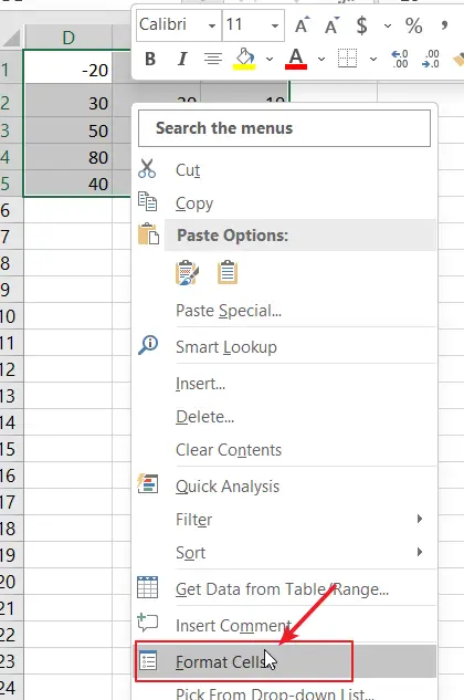
And for this, you can use the paste special option. Wondering how? Let me tell you. In the paste special option, there are “operation” options that you can use to perform some simple calculations. You can use these same options to make negative numbers positive without using any formula or adding any extra column. Just follow these steps.
- First of all, in any cell in your worksheet, enter -1.
- After that, copy it.
- Now, select the range of cells in which you have negative numbers.
- Right-Click ⇢ Paste Special ⇢ Operations ⇢ Multiply.
- In the end, click OK.
All the negative numbers are converted into positive ones.
The only thing you need to take care of is that this is not a dynamic method. So, you need to do it again and again if you frequently update your data. But this method is quick and easy to use, and you don’t need any formula.
4. Remove the Negative Sign with Flash Fill
I am sure you have used flash fill once in your lifetime and if not, you must use it, it’s a game-changer. This is an insane method to turn negative numbers into positive ones, here are the steps.
- First of all, in cell B2, enter the positive number for the negative number you have in cell A2.
- After that, come to cell B3 and press the shortcut key Ctrl + E.
- At this point, in the B column, you have all the numbers in positive form.
- Now, click on the small icon you have on the right side of column B and select “Accept Suggestions”.
Congratulations, you have converted all the negative numbers into positive ones with flash fill.
This method is also not a dynamic one, but quick and easy to use.
5. Apply Custom Formatting to Show as Positive Numbers
This is also a possibility that instead of converting a negative number you just want to show it as a positive number. And in this situation, you can use custom formatting. Here are the steps to this.
- First of all, select the range of the cells you need to convert into positive numbers.
- After that, press the shortcut key Ctrl + 1. It will open the custom formatting options.
- Now, go to “Custom” and in the type input bar, enter “#,###;#,###”.
- In the end, click OK.

This will show all the negative numbers as positive. But, in actuality these all are still negative numbers, just formatting is changed.

If you select a cell and look at the formula bar, you can check, that it’s still a negative number. So, when you use it in further calculation it will act as a negative number.
6. Run a VBA Code to Convert to Positive Numbers
If you are a VBA lover then you can use a simple code to reverse the sign of negative numbers instantly.
Sub numberP2N()

Dim myCell As Range

For Each myCell In Selection

    If myCell.Value <> "" Then

        If IsNumeric(myCell.Value) Then

            myCell.Value = Abs(myCell.Value)

        End If

    End If

Next myCell

End Sub
To use this code, you just need to select the range of negative numbers and run this macro.
First, it will check each cell of selection if there is a numeric value in it or not and then convert it to a positive value.
Once you run this code, you can’t undo your action.
Related: VBA Tutorial
7. Use Power Query to Convert Get Positive Numbers
Yes, you can use a power query to convert a negative number into a positive number and the best part is it’s a one-time setup. Just follow these simple steps.
- First of all, select any of the cells from the data range where you have negative numbers.

- After that, go to the Data tab ➜ From Table.

- It will convert the range into a table and load it in the power query editor.

- Now, right-click on the column, and go to Transform ➜ Absolute Value.

- In the end, in the power query editor, go to Home Tab ➜ Close ➜ Close and load.

Related: Power Query Tutorial
Conclusion
As I said, to turn a negative number into a positive number you don’t need to use rocket science. Even one method can be sufficient, but I have listed all these methods to help you to handle different situations.
I am sure you found all these methods helpful, but now, you have to tell me one thing.
Do you know any other method for this? Please share your views with me in the comment section. I’d love to hear from you and please don’t forget to share it with your friends, I am sure they will appreciate it.