
Заливка ячейки цветом в VBA Excel. Фон ячейки. Свойства .Interior.Color и .Interior.ColorIndex. Цветовая модель RGB. Стандартная палитра. Очистка фона ячейки.
Свойство .Interior.Color объекта Range
Начиная с Excel 2007 основным способом заливки диапазона или отдельной ячейки цветом (зарисовки, добавления, изменения фона) является использование свойства .Interior.Color объекта Range путем присваивания ему значения цвета в виде десятичного числа от 0 до 16777215 (всего 16777216 цветов).
Заливка ячейки цветом в VBA Excel
Пример кода 1:
|
Sub ColorTest1() Range(«A1»).Interior.Color = 31569 Range(«A4:D8»).Interior.Color = 4569325 Range(«C12:D17»).Cells(4).Interior.Color = 568569 Cells(3, 6).Interior.Color = 12659 End Sub |
Поместите пример кода в свой программный модуль и нажмите кнопку на панели инструментов «Run Sub» или на клавиатуре «F5», курсор должен быть внутри выполняемой программы. На активном листе Excel ячейки и диапазон, выбранные в коде, окрасятся в соответствующие цвета.
Есть один интересный нюанс: если присвоить свойству .Interior.Color отрицательное значение от -16777215 до -1, то цвет будет соответствовать значению, равному сумме максимального значения палитры (16777215) и присвоенного отрицательного значения. Например, заливка всех трех ячеек после выполнения следующего кода будет одинакова:
|
Sub ColorTest11() Cells(1, 1).Interior.Color = —12207890 Cells(2, 1).Interior.Color = 16777215 + (—12207890) Cells(3, 1).Interior.Color = 4569325 End Sub |
Проверено в Excel 2016.
Вывод сообщений о числовых значениях цветов
Числовые значения цветов запомнить невозможно, поэтому часто возникает вопрос о том, как узнать числовое значение фона ячейки. Следующий код VBA Excel выводит сообщения о числовых значениях присвоенных ранее цветов.
Пример кода 2:
|
Sub ColorTest2() MsgBox Range(«A1»).Interior.Color MsgBox Range(«A4:D8»).Interior.Color MsgBox Range(«C12:D17»).Cells(4).Interior.Color MsgBox Cells(3, 6).Interior.Color End Sub |
Вместо вывода сообщений можно присвоить числовые значения цветов переменным, объявив их как Long.
Использование предопределенных констант
В VBA Excel есть предопределенные константы часто используемых цветов для заливки ячеек:
| Предопределенная константа | Наименование цвета |
|---|---|
| vbBlack | Черный |
| vbBlue | Голубой |
| vbCyan | Бирюзовый |
| vbGreen | Зеленый |
| vbMagenta | Пурпурный |
| vbRed | Красный |
| vbWhite | Белый |
| vbYellow | Желтый |
| xlNone | Нет заливки |
Присваивается цвет ячейке предопределенной константой в VBA Excel точно так же, как и числовым значением:
Пример кода 3:
|
Range(«A1»).Interior.Color = vbGreen |
Цветовая модель RGB
Цветовая система RGB представляет собой комбинацию различных по интенсивности основных трех цветов: красного, зеленого и синего. Они могут принимать значения от 0 до 255. Если все значения равны 0 — это черный цвет, если все значения равны 255 — это белый цвет.
Выбрать цвет и узнать его значения RGB можно с помощью палитры Excel:

Палитра Excel
Чтобы можно было присвоить ячейке или диапазону цвет с помощью значений RGB, их необходимо перевести в десятичное число, обозначающее цвет. Для этого существует функция VBA Excel, которая так и называется — RGB.
Пример кода 4:
|
Range(«A1»).Interior.Color = RGB(100, 150, 200) |
Список стандартных цветов с RGB-кодами смотрите в статье: HTML. Коды и названия цветов.
Очистка ячейки (диапазона) от заливки
Для очистки ячейки (диапазона) от заливки используется константа xlNone:
|
Range(«A1»).Interior.Color = xlNone |
Свойство .Interior.ColorIndex объекта Range
До появления Excel 2007 существовала только ограниченная палитра для заливки ячеек фоном, состоявшая из 56 цветов, которая сохранилась и в настоящее время. Каждому цвету в этой палитре присвоен индекс от 1 до 56. Присвоить цвет ячейке по индексу или вывести сообщение о нем можно с помощью свойства .Interior.ColorIndex:
Пример кода 5:
|
Range(«A1»).Interior.ColorIndex = 8 MsgBox Range(«A1»).Interior.ColorIndex |
Просмотреть ограниченную палитру для заливки ячеек фоном можно, запустив в VBA Excel простейший макрос:
Пример кода 6:
|
Sub ColorIndex() Dim i As Byte For i = 1 To 56 Cells(i, 1).Interior.ColorIndex = i Next End Sub |
Номера строк активного листа от 1 до 56 будут соответствовать индексу цвета, а ячейка в первом столбце будет залита соответствующим индексу фоном.
Подробнее о стандартной палитре Excel смотрите в статье: Стандартная палитра из 56 цветов, а также о том, как добавить узор в ячейку.
Содержание
- Описание работы функции
- Пример использования
- Свойство .Interior.Color объекта Range
- Заливка ячейки цветом в VBA Excel
- Вывод сообщений о числовых значениях цветов
- Форматирование диапазона
- Нажатие кнопки Enter
- Вставка символа
- Добавление дополнительного символа
- Коды различных цветов в MS Excel 2003
Описание работы функции
Функция =ЦВЕТЗАЛИВКИ(ЯЧЕЙКА) возвращает код цвета заливки выбранной ячейки. Имеет один обязательный аргумент:
- ЯЧЕЙКА – ссылка на ячейку, для которой необходимо применить функцию.
Ниже представлен пример, демонстрирующий работу функции.

Следует обратить внимание на тот факт, что функция не пересчитывается автоматически. Это связано с тем, что изменение цвета заливки ячейки Excel не приводит к пересчету формул. Для пересчета формулы необходимо пользоваться сочетанием клавиш Ctrl+Alt+F9
Пример использования
Так как заливка ячеек значительно упрощает восприятие данных, то пользоваться ей любят практически все пользователи. Однако есть и большой минус – в стандартном функционале Excel отсутствует возможность выполнять операции на основе цвета заливки. Нельзя просуммировать ячейки определенного цвета, посчитать их количество, найти максимальное и так далее.
С помощью функции ЦВЕТЗАЛИВКИ все это становится выполнимым. Например, “протяните” данную формулу с цветом заливки в соседнем столбце и производите вычисления на основе числового кода ячейки.
Свойство .Interior.Color объекта Range
Начиная с Excel 2007 основным способом заливки диапазона или отдельной ячейки цветом (зарисовки, добавления, изменения фона) является использование свойства .Interior.Color объекта Range путем присваивания ему значения цвета в виде десятичного числа от 0 до 16777215 (всего 16777216 цветов).
Заливка ячейки цветом в VBA Excel
Пример кода 1:
|
Sub ColorTest1() Range(“A1”).Interior.Color = 31569 Range(“A4:D8”).Interior.Color = 4569325 Range(“C12:D17”).Cells(4).Interior.Color = 568569 Cells(3, 6).Interior.Color = 12659 End Sub |
Поместите пример кода в свой программный модуль и нажмите кнопку на панели инструментов «Run Sub» или на клавиатуре «F5», курсор должен быть внутри выполняемой программы. На активном листе Excel ячейки и диапазон, выбранные в коде, окрасятся в соответствующие цвета.
Есть один интересный нюанс: если присвоить свойству .Interior.Color отрицательное значение от -16777215 до -1, то цвет будет соответствовать значению, равному сумме максимального значения палитры (16777215) и присвоенного отрицательного значения. Например, заливка всех трех ячеек после выполнения следующего кода будет одинакова:
|
Sub ColorTest11() Cells(1, 1).Interior.Color = –12207890 Cells(2, 1).Interior.Color = 16777215 + (–12207890) Cells(3, 1).Interior.Color = 4569325 End Sub |
Вывод сообщений о числовых значениях цветов
Числовые значения цветов запомнить невозможно, поэтому часто возникает вопрос о том, как узнать числовое значение фона ячейки. Следующий код VBA Excel выводит сообщения о числовых значениях присвоенных ранее цветов.
Пример кода 2:
|
Sub ColorTest2() MsgBox Range(“A1”).Interior.Color MsgBox Range(“A4:D8”).Interior.Color MsgBox Range(“C12:D17”).Cells(4).Interior.Color MsgBox Cells(3, 6).Interior.Color End Sub |
Вместо вывода сообщений можно присвоить числовые значения цветов переменным, объявив их как Long.
Форматирование диапазона
Самый известный способ поставить прочерк в ячейке – это присвоить ей текстовый формат. Правда, этот вариант не всегда помогает.
- Выделяем ячейку, в которую нужно поставить прочерк. Кликаем по ней правой кнопкой мыши. В появившемся контекстном меню выбираем пункт «Формат ячейки». Можно вместо этих действий нажать на клавиатуре сочетание клавиш Ctrl+1.
- Запускается окно форматирования. Переходим во вкладку «Число», если оно было открыто в другой вкладке. В блоке параметров «Числовые форматы» выделяем пункт «Текстовый». Жмем на кнопку «OK».

После этого выделенной ячейке будет присвоено свойство текстового формата. Все введенные в нее значения будут восприниматься не как объекты для вычислений, а как простой текст. Теперь в данную область можно вводить символ «-» с клавиатуры и он отобразится именно как прочерк, а не будет восприниматься программой, как знак «минус».

Существует ещё один вариант переформатирования ячейки в текстовый вид. Для этого, находясь во вкладке «Главная», нужно кликнуть по выпадающему списку форматов данных, который расположен на ленте в блоке инструментов «Число». Открывается перечень доступных видов форматирования. В этом списке нужно просто выбрать пункт «Текстовый».

Нажатие кнопки Enter
Но данный способ не во всех случаях работает. Зачастую, даже после проведения этой процедуры при вводе символа «-» вместо нужного пользователю знака появляются все те же ссылки на другие диапазоны. Кроме того, это не всегда удобно, особенно если в таблице ячейки с прочерками чередуются с ячейками, заполненными данными. Во-первых, в этом случае вам придется форматировать каждую из них в отдельности, во-вторых, у ячеек данной таблицы будет разный формат, что тоже не всегда приемлемо. Но можно сделать и по-другому.
- Выделяем ячейку, в которую нужно поставить прочерк. Жмем на кнопку «Выровнять по центру», которая находится на ленте во вкладке «Главная» в группе инструментов «Выравнивание». А также кликаем по кнопке «Выровнять по середине», находящейся в том же блоке. Это нужно для того, чтобы прочерк располагался именно по центру ячейки, как и должно быть, а не слева.
- Набираем в ячейке с клавиатуры символ «-». После этого не делаем никаких движений мышкой, а сразу жмем на кнопку Enter, чтобы перейти на следующую строку. Если вместо этого пользователь кликнет мышкой, то в ячейке, где должен стоять прочерк, опять появится формула.
Данный метод хорош своей простотой и тем, что работает при любом виде форматирования. Но, в то же время, используя его, нужно с осторожностью относиться к редактированию содержимого ячейки, так как из-за одного неправильного действия вместо прочерка может опять отобразиться формула.
Вставка символа
Ещё один вариант написания прочерка в Эксель – это вставка символа.
- Выделяем ячейку, куда нужно вставить прочерк. Переходим во вкладку «Вставка». На ленте в блоке инструментов «Символы» кликаем по кнопке «Символ».
- Находясь во вкладке «Символы», устанавливаем в окне поля «Набор» параметр «Символы рамок». В центральной части окна ищем знак «─» и выделяем его. Затем жмем на кнопку «Вставить».

После этого прочерк отразится в выделенной ячейке.

Существует и другой вариант действий в рамках данного способа. Находясь в окне «Символ», переходим во вкладку «Специальные знаки». В открывшемся списке выделяем пункт «Длинное тире». Жмем на кнопку «Вставить». Результат будет тот же, что и в предыдущем варианте.

Данный способ хорош тем, что не нужно будет опасаться сделанного неправильного движения мышкой. Символ все равно не изменится на формулу. Кроме того, визуально прочерк поставленный данным способом выглядит лучше, чем короткий символ, набранный с клавиатуры. Главный недостаток данного варианта – это потребность выполнить сразу несколько манипуляций, что влечет за собой временные потери.
Добавление дополнительного символа
Кроме того, существует ещё один способ поставить прочерк. Правда, визуально этот вариант не для всех пользователей будет приемлемым, так как предполагает наличие в ячейке, кроме собственно знака «-», ещё одного символа.
- Выделяем ячейку, в которой нужно установить прочерк, и ставим в ней с клавиатуры символ «‘». Он располагается на той же кнопке, что и буква «Э» в кириллической раскладке. Затем тут же без пробела устанавливаем символ «-».
- Жмем на кнопку Enter или выделяем курсором с помощью мыши любую другую ячейку. При использовании данного способа это не принципиально важно. Как видим, после этих действий на листе был установлен знак прочерка, а дополнительный символ «’» заметен лишь в строке формул при выделении ячейки.

Существует целый ряд способов установить в ячейку прочерк, выбор между которыми пользователь может сделать согласно целям использования конкретного документа. Большинство людей при первой неудачной попытке поставить нужный символ пытаются сменить формат ячеек. К сожалению, это далеко не всегда срабатывает. К счастью, существуют и другие варианты выполнения данной задачи: переход на другую строку с помощью кнопки Enter, использование символов через кнопку на ленте, применение дополнительного знака «’». Каждый из этих способов имеет свои достоинства и недостатки, которые были описаны выше. Универсального варианта, который бы максимально подходил для установки прочерка в Экселе во всех возможных ситуациях, не существует.
Коды различных цветов в MS Excel 2003
Коды различных цветов при использовании конструкции типа .Interior.ColorIndex. Бесцветный код: -4142

Источники
- https://micro-solution.ru/projects/addin_vba-excel/color_interior
- https://vremya-ne-zhdet.ru/vba-excel/tsvet-yacheyki-zalivka-fon/
- http://word-office.ru/kak-sdelat-chtoby-vmesto-nulya-byl-procherk-v-excel.html
- http://aqqew.blogspot.com/2011/03/ms-excel-2003.html
Change the Colors of Cells Using Excel Visual Basic
Interior (Background) Color:
The general format is:
Range("Cell_Range").Interior.Color = RGB(R, G, B)OR:
Range("Cell_Range").Interior.ColorIndex = index_IDFont Color:
The general format is:
Range("Cell_Range").Font.Color = RGB(R, G, B)OR
Range("Cell_Range").Font.ColorIndex = index_IDCell Border Color:
The general format is:
Range("Cell_Range").Borders.Color = RGB(R, G, B)OR
Range("Cell_Range").Borders.ColorIndex = 49OR
Range("Cell_Range").Borders(Which_Border).Color =RGB(R, G, B)Cell_Range indicates Which cells you want to be colored. (R,G,B) indicates how much (R)ed, (G)reen, and (B)lue you want to include in the color. Each RGB value has a maximum value of 255 and a minimum of 0. RGB(255,0,0) uses maximum red with no other colors, making the color red. RGB(0,255,0) uses no red or blue with a maximum green, making the color green. RGB(150,20,150) makes it this color.
index_ID is a pre-determined color that can be determined from this list: Color Options
Which_border, for the border colors, indicates the desired border to change the color of
Example 1: Change the Interior Color of a Cell
Private Sub CommandButton1_Click()Range("A1:A10").Interior.Color = RGB(255, 0, 0)Range("B1:B10").Interior.ColorIndex = 49End Sub
One line uses RGB values to set part of column “A” to a background of red. The other uses ColorIndex to change it to a blue color. It looks like the image below when executed.

Example 2: Change the Font Color of a Cell
Private Sub CommandButton1_Click()Range("A1:A10").Font.Color = RGB(255, 0, 0)Range("B1:B10").Font.ColorIndex = 49End Sub
The first line changes the font in part of column A to a red color. The second line uses ColorIndex to change the font in part of column B to a dark blue color.

Example 3: Change the Border Color of a Cell
Private Sub CommandButton1_Click()Range("A1:A10").Borders.Color = RGB(255, 0, 0)Range("B1:B10").Borders.ColorIndex = 49Range("D1:D10").Borders(xlLeft).Color = RGB(0, 0, 255)Range("D1:D10").Borders(xlBottom).Color = RGB(255, 0, 255)Range("E1:E10").Borders(xlRight).ColorIndex = 4Range("E1:E10").Borders(xlTop).ColorIndex = 51End Sub
The first line changes all the borders of the A column range to RGB(255,0,0), which is red. The second line uses colorIndex to change all the borders in the B column range to a dark blue. Lines 4 through 8 show specific borders being colored.

Example 4: Background, Font, and Border Color Change
Private Sub CommandButton1_Click()Range("A1:A10").Interior.Color = RGB(0, 0, 128)Range("A1:A10").Font.Color = RGB(255, 255, 255)Range("A1:A10").Borders.ColorIndex = 53End Sub
Some Possible Colors Choices: Color Options
| Color | Index_ID | R | G | B |
| 1 | 0 | 0 | 0 | |
| 2 | 255 | 255 | 255 | |
| 3 | 255 | 0 | 0 | |
| 4 | 0 | 255 | 0 | |
| 5 | 0 | 0 | 255 | |
| 6 | 255 | 255 | 0 | |
| 7 | 255 | 0 | 255 | |
| 8 | 0 | 255 | 255 | |
| 9 | 128 | 0 | 0 | |
| 10 | 0 | 128 | 0 | |
| 11 | 0 | 0 | 128 | |
| 12 | 128 | 128 | 0 | |
| 13 | 128 | 0 | 128 | |
| 14 | 0 | 128 | 128 | |
| 15 | 192 | 192 | 192 | |
| 16 | 128 | 128 | 128 | |
| 17 | 153 | 153 | 255 | |
| 18 | 153 | 51 | 102 | |
| 19 | 255 | 255 | 204 | |
| 20 | 204 | 255 | 255 | |
| 21 | 102 | 0 | 102 | |
| 22 | 255 | 128 | 128 | |
| 23 | 0 | 102 | 204 | |
| 24 | 204 | 204 | 255 | |
| 25 | 0 | 0 | 128 | |
| 26 | 255 | 0 | 255 | |
| 27 | 255 | 255 | 0 | |
| 28 | 0 | 255 | 255 | |
| 29 | 128 | 0 | 128 | |
| 30 | 128 | 0 | 0 | |
| 31 | 0 | 128 | 128 | |
| 32 | 0 | 0 | 255 | |
| 33 | 0 | 204 | 255 | |
| 34 | 204 | 255 | 255 | |
| 35 | 204 | 255 | 204 | |
| 36 | 255 | 255 | 153 | |
| 37 | 153 | 204 | 255 | |
| 38 | 255 | 153 | 204 | |
| 39 | 204 | 153 | 255 | |
| 40 | 255 | 204 | 153 | |
| 41 | 51 | 102 | 255 | |
| 42 | 51 | 204 | 204 | |
| 43 | 153 | 204 | 0 | |
| 44 | 255 | 204 | 0 | |
| 45 | 255 | 153 | 0 | |
| 46 | 255 | 102 | 0 | |
| 47 | 102 | 102 | 153 | |
| 48 | 150 | 150 | 150 | |
| 49 | 0 | 51 | 102 | |
| 50 | 51 | 153 | 102 | |
| 51 | 0 | 51 | 0 | |
| 52 | 51 | 51 | 0 | |
| 53 | 153 | 51 | 0 | |
| 54 | 153 | 51 | 102 | |
| 55 | 51 | 51 | 153 | |
| 56 | 51 | 51 | 51 |
Excel VBA Resources
Applies to: Microsoft Excel 365, 2021, 2019, 2016.
In today’s VBA for Excel Automation tutorial we’ll learn about how we can programmatically change the color of a cell based on the cell value.
We can use this technique when developing a dashboard spreadsheet for example.
Step #1: Prepare your spreadsheet
If you are not yet developing on Excel, we’d recommend to look into our introductory guide to Excel Macros. You also need to make sure that the Developer tab is available in your Microsoft Excel Ribbon, as you’ll use it to write some simple code.
- Open Microsoft Excel. Note that code provided in this tutorial is expected to function in Excel 2007 and beyond.
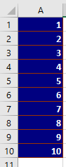
- In an empty worksheet, add the following table :

- Now go ahead and define a named Range by hitting: Formulas>>Define Name
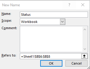
- Hit OK
Step #2: Changing cell interior color based on value with Cell.Interior.Color
- Hit the Developer entry in the Ribbon.
- Hit Visual Basic or Alt+F11 to open your developer VBA editor.
- Next highlight the Worksheet in which you would like to run your code. Alternatively, select a module that has your VBA code.
- Go ahead and paste this code. In our example we’ll modify the interior color of a range of cells to specific cell RGB values corresponding to the red, yellow and green colors.
- Specifically we use the Excel VBA method Cell.Interior.Color and pass the corresponding RGB value or color index.
Sub Color_Cell_Condition()

Dim MyCell As Range
Dim StatValue As String
Dim StatusRange As Range

Set StatusRange = Range("Status")

For Each MyCell In StatusRange

StatValue = MyCell.Value
Select Case StatValue

    Case "Progressing"
    MyCell.Interior.Color = RGB(0, 255, 0)

    Case "Pending Feedback"
    MyCell.Interior.Color = RGB(255, 255, 0)

    Case "Stuck"
    MyCell.Interior.Color = RGB(255, 0, 0)

End Select

Next MyCell

End Sub- Run your code – either by pressing on F5 or Run>> Run Sub / UserForm.
- You’ll notice the status dashboard was filled as shown below:

- Save your code and close your VBA editor.
I need to highlight the cells with wrong data in excel with golden color which I am able to do. But as soon as the user corrects the data and clicks on validate button the interior color should be revert back to original interior color. This is not happening. Please point out the error. And please suggest exact code because I’ve tried many thing but nothing has worked so far.
private void ValidateButton_Click(object sender, RibbonControlEventArgs e)
      {
          bool LeftUntagged = false;
          Excel.Workbook RawExcel = Globals.ThisAddIn.Application.ActiveWorkbook;
          Excel.Worksheet sheet = null;
          Excel.Range matrix = sheet.UsedRange;
          for (int x = 1; x <= matrix.Rows.Count; x++)
          {
              for (int y = 1; y <= matrix.Columns.Count; y++)
              {
                  string CellColor = sheet.Cells[x, y].Interior.Color.ToString();
                  if (sheet.Cells[x, y].Value != null && (Excel.XlRgbColor.rgbGold.Equals(sheet.Cells[x, y].Interior.Color) || Excel.XlRgbColor.rgbWhite.Equals(sheet.Cells[x, y].Interior.Color)))
                  {
                      sheet.Cells[x, y].Interior.Color = Color.Transparent;
                  }
              }
          }
      }
asked Aug 13, 2013 at 14:10
![]()
I achieved what I was trying to do. Here is the solution:
private void ValidateButton_Click(object sender, RibbonControlEventArgs e)
      {
          bool LeftUntagged = false;
          Excel.Workbook RawExcel = Globals.ThisAddIn.Application.ActiveWorkbook;
          Excel.Worksheet sheet = null;
          Excel.Range matrix = sheet.UsedRange;
          for (int x = 1; x <= matrix.Rows.Count; x++)
          {
              for (int y = 1; y <= matrix.Columns.Count; y++)
              {
                  string CellColor = sheet.Cells[x, y].Interior.Color.ToString(); //Here I go double value which is converted to string.
                  if (sheet.Cells[x, y].Value != null && (CellColor == Color.Transparent.ToArgb().ToString() || **CellColor == Excel.XlRgbColor.rgbGold.GetHashCode().ToString()**))
                  {
                      sheet.Cells[x, y].Interior.Color = Color.Transparent;
                  }
              }
          }
      }
![]()
davidsbro
2,7614 gold badges22 silver badges33 bronze badges
answered Aug 14, 2013 at 12:35
![]()
1
Try:
sheet.Cells[x, y].Interior.ColorIndex = -4142; //xlNone
answered Aug 13, 2013 at 14:20
![]()
Richard MorganRichard Morgan
7,5819 gold badges49 silver badges86 bronze badges
1
The way to do this is to use the ColorIndex. A full list of values can be found at Adding Color to Excel 2007 Worksheets by Using the ColorIndex Property.
In the code, just use the index from figure 1 in the link above.
// For example
sheet.Cells[x, y].Interior.ColorIndex = 3; // Set to RED
If you need to compare colors, you can simply compare the ColorIndex value
answered Aug 13, 2013 at 14:27
![]()
SwDevMan81SwDevMan81
48.6k22 gold badges149 silver badges183 bronze badges
(too large for a comment)
So you want to colour a cell, based on its contents, compared to some other cell’s contents. In order to achieve that, you have created a macro which you need to launch in order to see its results.
Instead of that, I’d advise you to use conditional formatting. It does exactly what you want and there’s no need for launching a macro anymore, it all happens immediately.
Can you give an example of what you call «wrong data», I might try to find the condition, needed for configuring the conditional formatting.
answered Feb 3, 2022 at 8:48
![]()
DominiqueDominique
15.9k15 gold badges52 silver badges104 bronze badges
Change Background Color of Cell Range in Excel VBA
Description:
It is an interesting feature in excel, we can change background color of Cell, Range in Excel VBA. Specially, while preparing reports or dashboards, we change the backgrounds to make it clean and get the professional look to our projects.
Change Background Color of Cell Range in Excel VBA – Solution(s):
![]()
We can use Interior.Color OR Interior.ColorIndex properties of a Rage/Cell to change the background colors.
Change Background Color of Cell Range in Excel VBA – Examples
The following examples will show you how to change the background or interior color in Excel using VBA.
Example 1
In this Example below I am changing the Range B3 Background Color using Cell Object
Sub sbRangeFillColorExample1()

'Using Cell Object
Cells(3, 2).Interior.ColorIndex = 5 ' 5 indicates Blue Color

End Sub
Example 2
In this Example below I am changing the Range B3 Background Color using Range Object
Sub sbRangeFillColorExample2()

'Using Range Object
Range("B3").Interior.ColorIndex = 5

End Sub
Example 3
We can also use RGB color format, instead of ColorIndex. See the following example:
Sub sbRangeFillColorExample3()
'Using Cell Object
Cells(3, 2).Interior.Color = RGB(0, 0, 250)

'Using Range Object
Range("B3").Interior.Color = RGB(0, 0, 250)

End Sub
Example 4
The following example will apply all the colorIndex form 1 to 55 in Activesheet.
Sub sbPrintColorIndexColors()
Dim iCntr

For iCntr = 1 To 56
    Cells(iCntr, 1).Interior.ColorIndex = iCntr
    Cells(iCntr, 1) = iCntr
Next iCntr

End Sub
Instructions:
- Open an excel workbook
- Press Alt+F11 to open VBA Editor
- Insert a new module from Insert menu
- Copy the above code and Paste in the code window
- Save the file as macro enabled workbook
- Press F5 to execute the procedure
- You can see the interior colors are changing as per our code
Change Background Color of Cell Range in Excel VBA – Download: Example File
Here is the sample screen-shot of the example file.
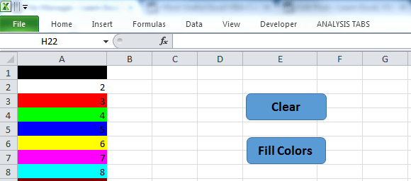
Download the file and explore how to change the interior or background colors in Excel using VBA.
ANALYSIS TABS – ColorIndex
A Powerful & Multi-purpose Templates for project management. Now seamlessly manage your projects, tasks, meetings, presentations, teams, customers, stakeholders and time. This page describes all the amazing new features and options that come with our premium templates.
Save Up to 85% LIMITED TIME OFFER

All-in-One Pack
120+ Project Management Templates
Essential Pack
50+ Project Management Templates
Excel Pack
50+ Excel PM Templates
PowerPoint Pack
50+ Excel PM Templates
MS Word Pack
25+ Word PM Templates
Ultimate Project Management Template
Ultimate Resource Management Template
Project Portfolio Management Templates
Related Posts
VBA Reference
Effortlessly
Manage Your Projects
120+ Project Management Templates
Seamlessly manage your projects with our powerful & multi-purpose templates for project management.
120+ PM Templates Includes:
3 Comments
-
Harbinder Singh
April 13, 2017 at 12:23 PM — Replyneed help in excel
In company there are 10000 employee and all having duty in A shift, B shift, C shift. Each shift of 08 hrs
i have to find those employee who work continuous 10 days or more then 10 days
please help me to find the solution using VB macro in excel or any other way to find from huge no of data in excel
Kindly provide me the solution.
-
RandomOne
May 23, 2017 at 5:46 AM — ReplyHarbinder Singh
its dependes of your database, can check with a vba code for filter based on the criteria, select the range and then color it,
Regards! -
Ken Schleede
July 10, 2019 at 6:44 AM — ReplyThanks! This is excellent. It allows me to control the colors much more reliably than conditional formatting.
Effectively Manage Your
Projects and Resources
ANALYSISTABS.COM provides free and premium project management tools, templates and dashboards for effectively managing the projects and analyzing the data.
We’re a crew of professionals expertise in Excel VBA, Business Analysis, Project Management. We’re Sharing our map to Project success with innovative tools, templates, tutorials and tips.
Project Management
Excel VBA
Download Free Excel 2007, 2010, 2013 Add-in for Creating Innovative Dashboards, Tools for Data Mining, Analysis, Visualization. Learn VBA for MS Excel, Word, PowerPoint, Access, Outlook to develop applications for retail, insurance, banking, finance, telecom, healthcare domains.
Page load link
Go to Top
In this article, let’s look at the various ways to set or remove the interior/background color of a cell or range – ie to fill the cell. We’ll also have a look at how to fill a cell/range with a pattern. Finally, we’ll review how to get the color input from the user using xlDialogEditColor and working with color gradients.
Example 1: Set the color of a cell / range
The .Interior.Color property is used to set the color of a cell or a range. There are various methods in which we can do this.
'Using XlRgbColor Enumeration - for few cells in a row
Range("B2:D2").Interior.Color = rgbDarkGreen

'Using Color Constants - for a cell using row and column number
Cells(3, 2).Interior.Color = vbYellow

'Specifying the RGB values - using A1 notation
Range("B4").Interior.Color = RGB(255, 0, 0)

'Using Color Code - for few cells in a column
Range("B5:B6").Interior.Color = 15773696

'Using Color Index - for a range
Range("B7:D8").Interior.ColorIndex = 7
This is how the output will look

For more details, refer to article Excel VBA, Cell Fill Color
Example 2: Set the color of a an entire row
You can use the .Interior.Color property on an entire row. Say you want to highlight all rows where the value of a column satisfies a condition:
Sub highlightRows()
    Dim rowNo As Integer
    For rowNo = 3 To 12
        If Sheet1.Cells(rowNo, 3).Value < 30 Then
            Rows(rowNo).Interior.Color = vbRed
        End If
    Next
End Sub
Here is the Excel before and after executing the code.

Example 3: Set the color of a an entire column
Similar to Example 2, you can fill an entire column using:
'Set color for column
Columns(2).Interior.Color = vbCyan
Example 4: Remove the color from a cell / range
You can also remove the background color of a cell by setting it to xlNone
'Remove color
Range("A1").Interior.Color = xlNone
or you can set a cell to have automatic color using xlColorIndexAutomatic
'Set color to automatic
Range("A1").Interior.ColorIndex = xlColorIndexAutomatic
Example 5: Get the color code of a cell
You can also get the color code of a cell. The line below gets the color code of the color used to fill cell A1 and prints it in cell B1:
'gets the color code used to fill cell A1
Cells(1, 2) = Range("A1").Interior.Color
Example 6: Get the color input from the user using xlDialogEditColor
The xlDialogEditColor is a dialog used to get a color code from the user. This dialog has 2 tabs: Standard and which we will see soon.
Syntax:
intResult = Application.Dialogs(xlDialogEditColor).Show(intIndex, [intRed], [intGreen], [intBlue])
intResult: Zero if the user cancels the dialog and -1 if the user selects a color.
intIndex: Selected color when the edit color dialog is opened. It is also used as an identifier to get the value of the color selected by the user. (More details below).
intRed, intGreen, intBlue: Red, blue and green components of a color
There are 2 methods for calling this dialog:
1. Displaying the standard tab: If only the intIndex is specified and the last 3 parameters are omitted, standard tab will be displayed. intIndex will decide the color index initially selected in the standard tab. This is a number between zero and 56.
intResult = Application.Dialogs(xlDialogEditColor).Show(20)

2. The custom tab is initially displayed. If all the 4 parameters, including the RGB values, are specified, the custom tab will be displayed.
intResult = Application.Dialogs(xlDialogEditColor).Show(20, 100, 100, 200)

So, here is the complete code to get the color code from the user:
Sub changeColor()

Dim intResult As Long, intColor As Long

'displays the color dialog
intResult = Application.Dialogs(xlDialogEditColor).Show(40, 100, 100, 200)

'gets the color selected by the user
intColor = ThisWorkbook.Colors(40)

'changes the fill color of cell A1
Range("A1").Interior.Color = intColor

End Sub
Note: The intIndex specified in the xlDialogEditColor (40 in our example) is also the index used by ThisWorkbook.Colors. You need to make sure that these two numbers match.
Example 7: Gradient’s Colors
You can create a gradient using “xlPatternLinearGradient”
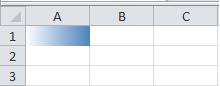
Range("A1").Interior.Pattern = xlPatternLinearGradient
It will look like this:
A gradient can have one or more colorStops, and each ColorStop has a position (a value between 0 and 1) and a color property. When you create a gradient, by default, the gradient has two ColorStop objects. One of the color stop objects has the position 1 and the other has the position 2. In order to be able to fully use the gradient properties in VBA, it is best to change the default positions to 0 and 1. In this way we would be able to have additional positions (colorStops) in between (i.e 0.5, 0.3). Let us now look at an example.
Sub multiColorStops()
Dim objColorStop As ColorStop
Dim lngColor1 As Long

'First create a gradient
Range("A1").Interior.Pattern = xlPatternLinearGradient

'Changes orientation to vertical (default is horizontal) - optional
Range("A1").Interior.Gradient.Degree = 90

'Clears all previous colorStop objects as they are at position 1 and 2
Range("A1").Interior.Gradient.ColorStops.Clear

'Start creating multiple colorStops at various positions from 0 to 1
Set objColorStop = Range("A1").Interior.Gradient.ColorStops.Add(0)

'Set the color for each colorstop
objColorStop.Color = vbYellow

Set objColorStop = Range("A1").Interior.Gradient.ColorStops.Add(0.33)
objColorStop.Color = vbRed

Set objColorStop = Range("A1").Interior.Gradient.ColorStops.Add(0.66)
objColorStop.Color = vbGreen

Set objColorStop = Range("A1").Interior.Gradient.ColorStops.Add(1)
objColorStop.Color = vbBlue

End Sub
The final result will look like this.

For more details, please refer to the article Excel VBA, Gradient’s Colors
Example 8: Color Patterns
Using VBA, you can also apply various patterns to cells in Excel. The patterns available can be seen in the snapshot below (Right click on a Cell > Format Cells > Fill tab > Pattern Style):

The pattern of a cell can be changed using the xlPattern enumeration. The code below changes the pattern of cell A1 to the checker pattern:
range("A1").Interior.Pattern = XlPattern.xlPatternChecker
Result:

You can also change the color of the pattern using the code below:
Range("A1").Interior.PatternColor = vbBlue
Result:

You can get a complete list of the XlPattern Enumeration in Excel here.
To get the index (as specified in the link above) of the pattern applied in a cell use:
MsgBox Range("A1").Interior.Pattern
It will display 9 for the checker pattern that we have applied earlier
For more details, refer to the article Excel VBA, Fill Pattern