
Содержание
- Способ 1: Меню «Таблицы»
- Способ 2: Копирование из Word
- Способ 3: Копирование из Excel
- Вопросы и ответы

Примечание: Все действия, представленные в статье, выполняются в версиях программы Microsoft Excel 2013 – 2021 годов, в связи с чем некоторые наименования элементов интерфейса и их месторасположение в других редакциях может отличаться.
Способ 1: Меню «Таблицы»
Несмотря на то что Excel по умолчанию является табличным процессором, в рабочую область программы можно вставить таблицу. Этот метод подразумевает быстрое форматирование заполненного диапазона данных для упорядочения и анализа связанных значений. Для этого потребуется проделать следующие действия:
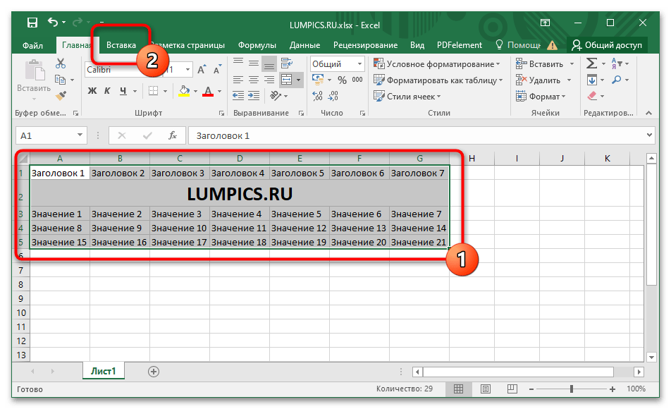
- Выделите область данных, которую необходимо преобразовать в таблицу, после чего откройте вкладку «Вставка».
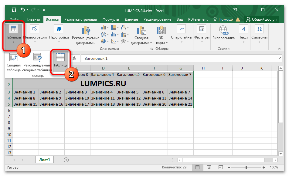
- На панели инструментов в блоке «Таблицы» выберите опцию «Таблица». Это же действие можно произвести посредством горячих клавиш Ctrl + T.
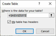
- В появившемся диалоговом окне удостоверьтесь, что диапазон данных выделен верно, установите при необходимости отметку «Таблица с заголовками» и кликните по кнопке «ОК».

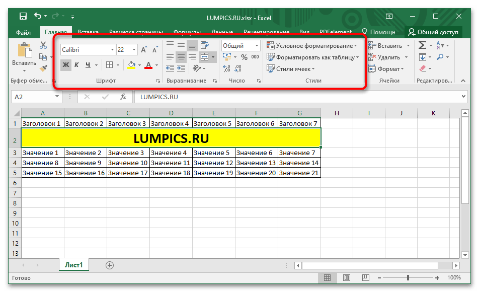
Сразу после этого таблица будет вставлена в Excel. Стоит отметить, что выполненное форматирование в некоторых случаях может отличаться от желаемого, и в таком случае потребуется произвести настройку вручную. На эту тему есть отдельная статья, в которой подробно описано использование всех соответствующих инструментов программы.
Подробнее: Принципы форматирования таблиц в Microsoft Excel
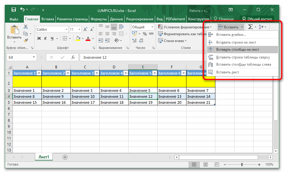
Обратите внимание! Можно пойти от обратного, сначала вставив таблицу в приложение, а затем заполонив все ее ячейки данными. В случае недостачи строк или столбцов следует выполнить их добавление. Этот процесс подробно разобран в другом материале на сайте.
Подробнее: Как добавить столбцы / строки в программу Microsoft Excel
Способ 2: Копирование из Word
При необходимости перенести таблицу из текстового редактора Word в Excel можно воспользоваться стандартными инструментами копирования, но итоговый результат будет зависеть от метода вставки. Альтернативный метод подразумевает применение функции импорта, процесс довольно трудоемкий, зато он позволяет произвести гибкую настройку перемещаемых данных, что актуально при работе с большим объемом информации. Оба упомянутых решения детально разобраны в отдельной статье на нашем сайте, с которой и рекомендуем ознакомиться.
Подробнее: Вставка таблицы из программы Word в Microsoft Excel

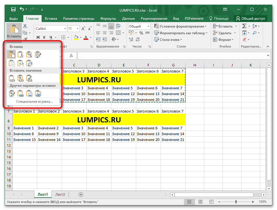
При переносе диапазона данных из одной книги в другую тоже используются штатные инструменты копирования, но в сравнении с ранее рассмотренным методом их значительно больше. Доступно пять способов перемещения значений, каждый из которых отличается алгоритмом выполнения и конечным результатом.
Подробнее: Копирование таблицы в Microsoft Excel
Стоит отметить, что применение специальной вставки не ограничивается теми случаями, которые описаны в вышеприведенной статье. Имеется гораздо больше возможностей, и все они были рассмотрены в представленной по ссылке ниже инструкции.
Подробнее: Применение специальной вставки в Microsoft Excel
Еще статьи по данной теме:
Помогла ли Вам статья?
Create and format tables
Create and format a table to visually group and analyze data.
Note: Excel tables shouldn’t be confused with the data tables that are part of a suite of What-If Analysis commands (Forecast, on the Data tab). See Introduction to What-If Analysis for more information.

Try it!
-
Select a cell within your data.
-
Select Home > Format as Table.
-
Choose a style for your table.
-
In the Create Table dialog box, set your cell range.
-
Mark if your table has headers.
-
Select OK.
-
Insert a table in your spreadsheet. See Overview of Excel tables for more information.
-
Select a cell within your data.
-
Select Home > Format as Table.
-
Choose a style for your table.
-
In the Create Table dialog box, set your cell range.
-
Mark if your table has headers.
-
Select OK.
To add a blank table, select the cells you want included in the table and click Insert > Table.
To format existing data as a table by using the default table style, do this:
-
Select the cells containing the data.
-
Click Home > Table > Format as Table.
-
If you don’t check the My table has headers box, Excel for the web adds headers with default names like Column1 and Column2 above the data. To rename a default header, double-click it and type a new name.
Note: You can’t change the default table formatting in Excel for the web.
Want more?
Overview of Excel tables
Video: Create and format an Excel table
Total the data in an Excel table
Format an Excel table
Resize a table by adding or removing rows and columns
Filter data in a range or table
Convert a table to a range
Using structured references with Excel tables
Excel table compatibility issues
Export an Excel table to SharePoint
Need more help?
I need one cell that will contains sum of all items from another table. Is it possible to place that table into cell so I can expand and collapse table when I needed from that one cell?
asked May 17, 2010 at 20:58
![]()
In a word, no, you can’t. Even if you set a cell to be equal to the entire range on the table and set it to an array formula via Ctrl+Shift+Enter (for example: ={A1:B10}) that cell would still evaluate to the top-left value of the table when used in formulas.
Just take the table and stick it in a hidden range or sheet.
answered May 17, 2010 at 21:23
![]()
ktdrvktdrv
3,5723 gold badges30 silver badges45 bronze badges
It is possible!
You need to use a named range, and you can insert your table as an object into a cell.
(tested in Excel 2010)
answered Apr 16, 2013 at 6:07
![]()
2
Содержание
- Import data from Excel to SQL Server or Azure SQL Database
- List of methods
- Import and Export Wizard
- Integration Services (SSIS)
- OPENROWSET and linked servers
- Distributed queries
- Linked servers
- Prerequisite — Save Excel data as text
- The Import Flat File Wizard
- BULK INSERT command
- BCP tool
- Copy Wizard (ADF)
- Azure Data Factory
- Common errors
- Microsoft.ACE.OLEDB.12.0″ has not been registered
- Cannot create an instance of OLE DB provider «Microsoft.ACE.OLEDB.12.0» for linked server «(null)»
- The 32-bit OLE DB provider «Microsoft.ACE.OLEDB.12.0» cannot be loaded in-process on a 64-bit SQL Server
- The OLE DB provider «Microsoft.ACE.OLEDB.12.0» for linked server «(null)» reported an error.
- Cannot initialize the data source object of OLE DB provider «Microsoft.ACE.OLEDB.12.0» for linked server «(null)»
- How to insert data from Excel to SQL Server
- Table of contents
- Background
- How to import data from Excel to SQL Server – Copy and Paste method
- Step-by-step Instructions
- How to insert data from Excel to SQL Server with an identity column
- Copy and paste data from Excel to SQL Server Views
- Excel to SQL Server import on a remote machine
- Tips when copying and pasting data from Excel to SQL server
- Validating your data – start with one row of data
- Inserting NULL values from Excel into a SQL Server table
- Tables with computed columns
- How to get the column names from the table in SQL Server to Excel
- Excel to SQL Server performance
- Copy and paste – a quick reference
- How to import data from Excel to SQL Server – SQL Spreads method
- Install the SQL Spreads Add-In for Excel
- Connect to your SQL Server database
- Inserting new rows into SQL Server
- Updating existing data in SQL Server
- Other tools and techniques
- Summary – insert data from Excel to SQL Server
- Johannes Åkesson
Import data from Excel to SQL Server or Azure SQL Database
Applies to: SQL Server Azure SQL Database
There are several ways to import data from Excel files to SQL Server or to Azure SQL Database. Some methods let you import data in a single step directly from Excel files; other methods require you to export your Excel data as text (CSV file) before you can import it.
This article summarizes the frequently used methods and provides links for more detailed information. A complete description of complex tools and services like SSIS or Azure Data Factory is beyond the scope of this article. To learn more about the solution that interests you, follow the provided links.
List of methods
There are a number of methods to import data from Excel. You may need to install SQL Server Management Studio (SSMS) to use some of these tools.
You can use the following tools to import data from Excel:
| Export to text first (SQL Server and SQL Database) | Directly from Excel (SQL Server on-premises only) |
|---|---|
| Import Flat File Wizard | SQL Server Import and Export Wizard |
| BULK INSERT statement | SQL Server Integration Services (SSIS) |
| BCP | OPENROWSET function |
| Copy Wizard (Azure Data Factory) | |
| Azure Data Factory |
If you want to import multiple worksheets from an Excel workbook, you typically have to run any of these tools once for each sheet.
To learn more, see limitations and known issues for loading data to or from Excel files.
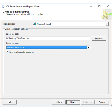
Import and Export Wizard
Import data directly from Excel files by using the SQL Server Import and Export Wizard. You also have the option to save the settings as a SQL Server Integration Services (SSIS) package that you can customize and reuse later.
In SQL Server Management Studio, connect to an instance of the SQL Server Database Engine.
Expand Databases.
Right-click a database.
Point to Tasks.
Choose to Import Data or Export Data:

This launches the wizard:
To learn more, review:
Integration Services (SSIS)
If you’re familiar with SQL Server Integration Services (SSIS) and don’t want to run the SQL Server Import and Export Wizard, create an SSIS package that uses the Excel Source and the SQL Server Destination in the data flow.
To learn more, review:
To start learning how to build SSIS packages, see the tutorial How to Create an ETL Package.

OPENROWSET and linked servers
In Azure SQL Database, you cannot import directly from Excel. You must first export the data to a text (CSV) file.
The ACE provider (formerly the Jet provider) that connects to Excel data sources is intended for interactive client-side use. If you use the ACE provider on SQL Server, especially in automated processes or processes running in parallel, you may see unexpected results.
Distributed queries
Import data directly into SQL Server from Excel files by using the Transact-SQL OPENROWSET or OPENDATASOURCE function. This usage is called a distributed query.
In Azure SQL Database, you cannot import directly from Excel. You must first export the data to a text (CSV) file.
Before you can run a distributed query, you have to enable the ad hoc distributed queries server configuration option, as shown in the following example. For more info, see ad hoc distributed queries Server Configuration Option.
The following code sample uses OPENROWSET to import the data from the Excel Sheet1 worksheet into a new database table.
Here’s the same example with OPENDATASOURCE .
To append the imported data to an existing table instead of creating a new table, use the INSERT INTO . SELECT . FROM . syntax instead of the SELECT . INTO . FROM . syntax used in the preceding examples.
To query the Excel data without importing it, just use the standard SELECT . FROM . syntax.
For more info about distributed queries, see the following topics:
- Distributed Queries (Distributed queries are still supported in SQL Server 2019, but the documentation for this feature has not been updated.)
- OPENROWSET
- OPENDATASOURCE
Linked servers
You can also configure a persistent connection from SQL Server to the Excel file as a linked server. The following example imports the data from the Data worksheet on the existing Excel linked server EXCELLINK into a new SQL Server database table named Data_ls .
You can create a linked server from SQL Server Management Studio, or by running the system stored procedure sp_addlinkedserver , as shown in the following example.
For more info about linked servers, see the following topics:
For more examples and info about both linked servers and distributed queries, see the following topic:
Prerequisite — Save Excel data as text
To use the rest of the methods described on this page — the BULK INSERT statement, the BCP tool, or Azure Data Factory — first you have to export your Excel data to a text file.
In Excel, select File | Save As and then select Text (Tab-delimited) (*.txt) or CSV (Comma-delimited) (*.csv) as the destination file type.
If you want to export multiple worksheets from the workbook, select each sheet and then repeat this procedure. The Save as command exports only the active sheet.
For best results with data importing tools, save sheets that contain only the column headers and the rows of data. If the saved data contains page titles, blank lines, notes, and so forth, you may see unexpected results later when you import the data.
The Import Flat File Wizard
Import data saved as text files by stepping through the pages of the Import Flat File Wizard.
As described previously in the Prerequisite section, you have to export your Excel data as text before you can use the Import Flat File Wizard to import it.
For more info about the Import Flat File Wizard, see Import Flat File to SQL Wizard.
BULK INSERT command
BULK INSERT is a Transact-SQL command that you can run from SQL Server Management Studio. The following example loads the data from the Data.csv comma-delimited file into an existing database table.
As described previously in the Prerequisite section, you have to export your Excel data as text before you can use BULK INSERT to import it. BULK INSERT can’t read Excel files directly. With the BULK INSERT command, you can import a CSV file that is stored locally or in Azure Blob storage.
For more info and examples for SQL Server and SQL Database, see the following topics:
BCP is a program that you run from the command prompt. The following example loads the data from the Data.csv comma-delimited file into the existing Data_bcp database table.
As described previously in the Prerequisite section, you have to export your Excel data as text before you can use BCP to import it. BCP can’t read Excel files directly. Use to import into SQL Server or SQL Database from a test (CSV) file saved to local storage.
For a text (CSV) file stored in Azure Blob storage, use BULK INSERT or OPENROWSET. For an examples, see Example.
For more info about BCP, see the following topics:
Copy Wizard (ADF)
Import data saved as text files by stepping through the pages of the Azure Data Factory (ADF) Copy Wizard.
As described previously in the Prerequisite section, you have to export your Excel data as text before you can use Azure Data Factory to import it. Data Factory can’t read Excel files directly.
For more info about the Copy Wizard, see the following topics:
Azure Data Factory
If you’re familiar with Azure Data Factory and don’t want to run the Copy Wizard, create a pipeline with a Copy activity that copies from the text file to SQL Server or to Azure SQL Database.
As described previously in the Prerequisite section, you have to export your Excel data as text before you can use Azure Data Factory to import it. Data Factory can’t read Excel files directly.
For more info about using these Data Factory sources and sinks, see the following topics:
To start learning how to copy data with Azure data factory, see the following topics:
Common errors
Microsoft.ACE.OLEDB.12.0″ has not been registered
This error occurs because the OLEDB provider is not installed. Install it from Microsoft Access Database Engine 2010 Redistributable. Be sure to install the 64-bit version if Windows and SQL Server are both 64-bit.
The full error is:
Cannot create an instance of OLE DB provider «Microsoft.ACE.OLEDB.12.0» for linked server «(null)»
This indicates that the Microsoft OLEDB has not been configured properly. Run the following Transact-SQL code to resolve this:
The full error is:
The 32-bit OLE DB provider «Microsoft.ACE.OLEDB.12.0» cannot be loaded in-process on a 64-bit SQL Server
This occurs when a 32-bit version of the OLD DB provider is installed with a 64-bit SQL Server. To resolve this issue, uninstall the 32-bit version and install the 64-bit version of the OLE DB provider instead.
The full error is:
The OLE DB provider «Microsoft.ACE.OLEDB.12.0» for linked server «(null)» reported an error.
Cannot initialize the data source object of OLE DB provider «Microsoft.ACE.OLEDB.12.0» for linked server «(null)»
Both of these errors typically indicate a permissions issue between the SQL Server process and the file. Ensure that the account that is running the SQL Server service has full access permission to the file. We recommend against trying to import files from the desktop.
Источник
How to insert data from Excel to SQL Server
In this article, you’re going to learn 2 easy ways to perform one of the most useful data management tasks: how to insert data from Excel to SQL Server.
Table of contents
- 1. Background
- 2. How to import data from Excel to SQL Server – Copy and Paste method
- a. Step-by-step instructions
- b. How to insert data from Excel to SQL Server with an identity column
- c. Copy and paste data from Excel to SQL Server Views
- d. Excel to SQL Server import on a remote machine
- e. Tips when copying and pasting data from Excel to SQL server
- f. Excel to SQL Server performance
- g. Copy and paste – a quick reference
- 3. How to import data from Excel to SQL Server – SQL Spreads method
- a. Install the SQL Spreads Add-In for Excel
- b. Connect to your database and insert data from Excel
- c. Inserting new rows into SQL Server
- d. Updating existing data in SQL Server
- 4. Other tools and techniques
- 5. Summary – insert data from Excel to SQL Server
Background
Before I founded SQL Spreads (an Excel Add-In to Import and Update SQL Server data from within Excel), I worked as a Business Intelligence consultant for many years using Microsoft’s BI-tools, such as SQL Server, SSIS, Reporting Services, Excel, etc.
I’ve found that when working on different projects, I tend to snap up a number of great-to-know things that I can re-use over and over again. One of these things that I re-use in almost every project is the ability to copy and paste data from Excel into a table in SQL Server.
It’s a really simple and convenient way to quickly import data into a table via SQL Server Management Studio. For example, populating a new dimension table, adding some test data, or inputting any other data that you need to quickly get into a table in SQL Server.
But what if you want to insert data from Excel to SQL without using Management Studio? What if there was a way to do this directly from Excel? This is where the SQL Spreads Excel Add-In that I’ve been working with over the last few years comes in. It makes your Excel to SQL Server import tasks much easier to do!
In this article, I’m therefore going to explain how to insert data from Excel to SQL Server using these 2 easy methods:
- Copy and paste from Excel to SQL tables via SQL Server Management Studio
- Insert directly from Excel to SQL tables using SQL Spreads
How to import data from Excel to SQL Server – Copy and Paste method
Step-by-step Instructions
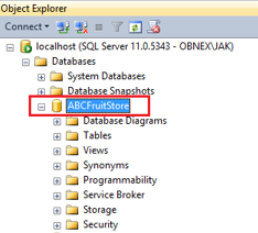
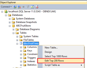
- Open SQL Server Management Studio and connect to your SQL Server database.
- Expand the Databases and the Tables folders for the table where you would like to insert your data from Excel.

- Right-click the table and select the fourth option – Edit Top 200 Rows.
- The data will be loaded and you will see the first 200 rows of data in the table.
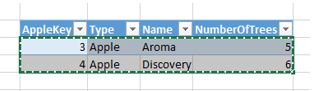
- Switch to Excel and select the rows and columns to insert from Excel to SQL Server.
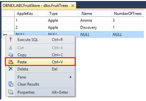
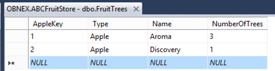
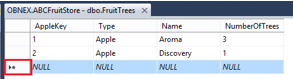
Right-click the selected cells and select Copy. - Switch back to SQL Server Management Studio and scroll down to the last row at the bottom and locate the row with a star in the left-most column.
- Right click the star in the column header and select Paste.
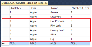
- You have now completed your SQL Server import, and your data from Excel is now in a table in SQL Server!


Remember: Always start with copying and pasting a single row of data from Excel to SQL Server. This is to check that there are no mismatches between your data from Excel and the SQL Server table (such as the number of columns) and that your data in Excel validates with the data types in the SQL Server table. See the section “Tips and tricks” below for more details.
How to insert data from Excel to SQL Server with an identity column
The same technique can also be used to copy and paste data into tables that have an auto-incrementing ID column (identity column).
The thing to keep in mind here is to also include an extra left-most blank column in Excel when copying the data from Excel to SQL Server. 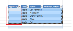
Follow these steps to copy and paste the data from Excel to SQL Server using a table with an auto-incrementing ID column:
- Open SQL Server Management Studio and connect to your SQL Server database.
- Expand the Databases and the Tables folders for the table where you would like to paste the Excel data.
- Right-click the table name and select Edit Top 200 Rows, the fourth option from the top.
- This will bring up a grid with the first 200 rows of data in the table.
- Switch to Excel and select the rows and columns to copy. Do not include the header row.
Now, also remember to include an extra blank left-most column in your selection.
Then, right-click the selected cells and select Copy. - Switch back to SQL Server Management Studio, and select the tab with the 200 rows from your table.
Go to the last row at the bottom and locate the row with a star in the left-most column. - Right-click on the star and select Paste.
- Your data from Excel is now pasted into your table in SQL Server, and SQL Server will automatically create the values in the ID/key column for you:

Copy and paste data from Excel to SQL Server Views
The copy and paste method also works when your Excel to SQL Server import is to a View as opposed to a Table. The only requirement is that the View should only contain data from one table.
In a View in SQL Server that contains data from several joined tables you cannot insert new rows, but you can update the data, as long as you only update columns that originate from the same base table.
Excel to SQL Server import on a remote machine
When working with SQL Server databases on a remote machine, where you connect to the remote machine using a Remote Desktop Connection, you can still use the same copy and paste technique to move the data from your local machine’s Excel to the SQL Server database on your remote machine.
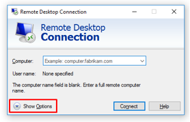
If you are not able to copy and paste the data into your SQL Server when connected using a Remote Desktop Connection, first check that copy and paste is enabled for the Remote Desktop Connection:
- Open the Remote Desktop Connection.
- Click the Show Options…
- Select the Local Resources tab, and then check that the Clipboard property is checked:
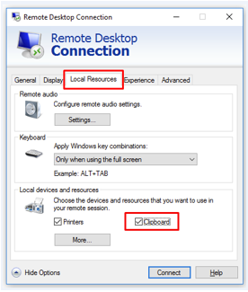
If you still cannot copy and paste data between Excel on your local machine and SQL Server on your remote database server, verify with your server administrator that the copy and paste feature is enabled for the Remote Desktop Connection on the server.
Tips when copying and pasting data from Excel to SQL server
Validating your data – start with one row of data
If the data that you copy from your Excel document does not match the data types of the columns in your SQL Server table, the inserting of the data will be canceled and you will get a warning message. This will happen for every row you paste from Excel to SQL Server. If you paste 500 rows from Excel with the wrong number of columns, you will get one warning message for each and every row that you paste.
To avoid this, the trick is to start to copy only a single row of data and paste it into the SQL Server table. If you get a warning message for incorrect data types, you can correct the mismatch and repeat the copy and paste procedure until all your Excel columns fit into the table in SQL Server. When all columns match, select the remaining rows and paste them all into the SQL Server table in one step.
Inserting NULL values from Excel into a SQL Server table
When you have columns in your SQL Server table that allow NULL values, and you want to insert a NULL value into the table, just enter the text NULL into the cell in Excel, and then copy and paste the data from Excel into SQL Server: 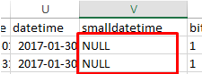
The NULL values will be inserted into the table in SQL Server: 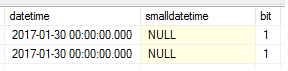
Tables with computed columns
For SQL Server tables containing computed columns, you can paste data from Excel into that table simply by leaving the data for the computed column blank in Excel, and then copying and pasting the data from Excel into the SQL Server table.
How to get the column names from the table in SQL Server to Excel
When you prepare the data in Excel for import into an existing SQL Server table, it is useful to have the column headings and a few rows of sample data as a reference in Excel.
There is a technique where you can copy existing data in SQL Server to Excel and include the table column names as header names.
Follow these steps to also include the column names when copying a few rows of data from a SQL Server table into Excel:
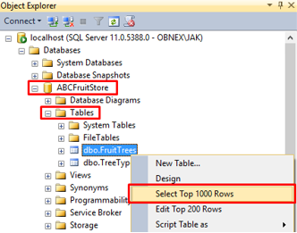
- In SQL Server Management Studio, locate your database and expand the Tables folder.
- Right-click your table name and select the third option – Select Top 1000 rows.
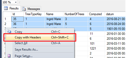
- Select the rows to copy to Excel by holding down the CTRL button and clicking the row numbers on the left side.
- When your rows are selected, right-click one row and select the Copy with Headers option:
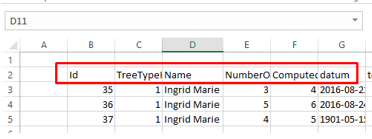
- Go to Excel and paste the data into a cell. The headers from the table in SQL Server will now be added as the first row:
Excel to SQL Server performance
Copying and pasting data from Excel to SQL Server is a really simple method to import data from Excel into your SQL Server database. One of the drawbacks is that it is not the fastest method if you need to insert larger amounts of data, such as several hundred thousand rows of data or more.
To get a reference to the performance limits, I have run a few tests on my local i7 machine with 8 GB of RAM with Microsoft Excel and SQL Server installed on the same machine.
I had the following results: copy data in Excel with 10 columns of mixed data types to SQL Server took about 2 seconds for 100 rows, about 30 seconds for 1000 rows, and about 10 minutes for 20,000 rows.
So, I would say that the limit to use the copy and paste feature is around a few thousand up to a few tens of thousands of rows of data. If you need to perform an Excel to SQL Server import with more data, then you should use the SQL Server Import and Export Wizard .
Copy and paste – a quick reference
- First, copy the data from Excel, and then paste it into the SQL Server table using the Database > Table > Edit top 200 rows menu option.
- Always start by copying and pasting a single row of data to validate the data types.
- For SQL Server tables with an identity column, add an extra blank left-most column before copying from Excel.
- Copy and paste from Excel to SQL Server can be used to insert up to a few tens of thousands of rows of data.
- To get the SQL Server column headers into Excel, right-click the table in SQL Server and select Copy with headers.
- Don’t forget that the technique also works great over Remote Desktop Connections!
How to import data from Excel to SQL Server – SQL Spreads method
This method is ideal for users that don’t want to insert data using SQL Server Management Studio.
Install the SQL Spreads Add-In for Excel
You can download a free trial of SQL Spreads from here .
- Run the SQLSpreadsSetup.exe file and follow the instructions.
- Restart Excel and accept the Add-In confirmation.
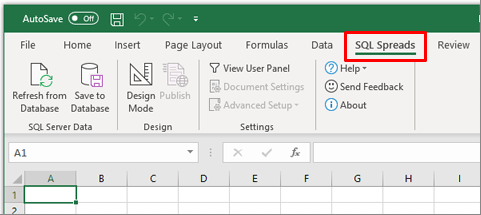
- You will find SQL Spreads in the tab menu in Excel:
For more details about installation, check out the Installing SQL Spreads section of our Knowledgebase.
Connect to your SQL Server database
Once SQL Spreads is installed, you’ll see that it has been added as a new ribbon tab.
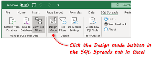
- Click on SQL Spreads and then click the Design Mode button
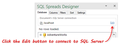
- In the SQL Spreads Designer panel on the right side, click the Edit button to open the SQL Server connection dialog.
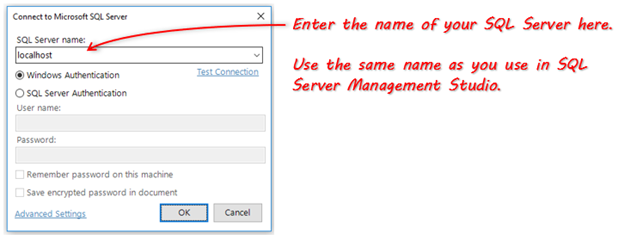
- Enter the name of your SQL Server into the SQL Server name field:
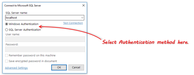
- Select if you should connect using your Windows-login (Windows Authentication) or enter a user name and password (SQL Server Authentication). Windows authentication is the more secure of the two options.
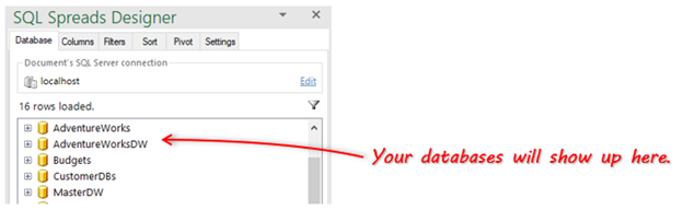
- Click OK. SQL Spreads will try to connect to the database. If the connection is successful, your databases will show up in the SQL Spreads Designer panel.
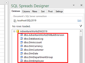
- Now that we’ve created the connection from Excel to SQL Server, we can select which table of data we want to use in Excel. In the SQL Spreads Designer, click on the database and then select your table.
As soon as you select a table, the data in the table is populated in the Excel sheet. You can now see all the data in your SQL Server table and use it in your Excel workbook. The real power with SQL Spreads is the ability to update or add to the data in SQL Server direct from Excel.
Inserting new rows into SQL Server
To import new data into SQL Server, scroll down to the first empty row and either type in your new data or paste a set of rows copied from another Excel workbook:
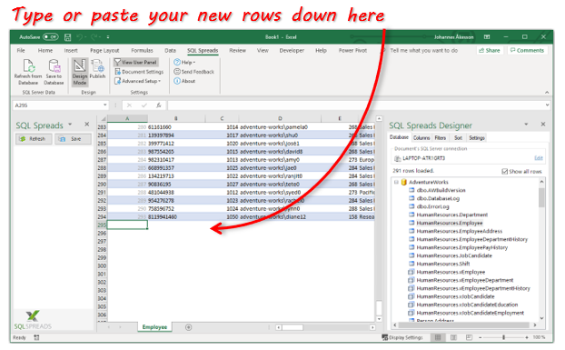
Once you’ve added or pasted the new rows, click the ‘Save to Database’ button to get the changes written to the table in SQL Server.
Updating existing data in SQL Server
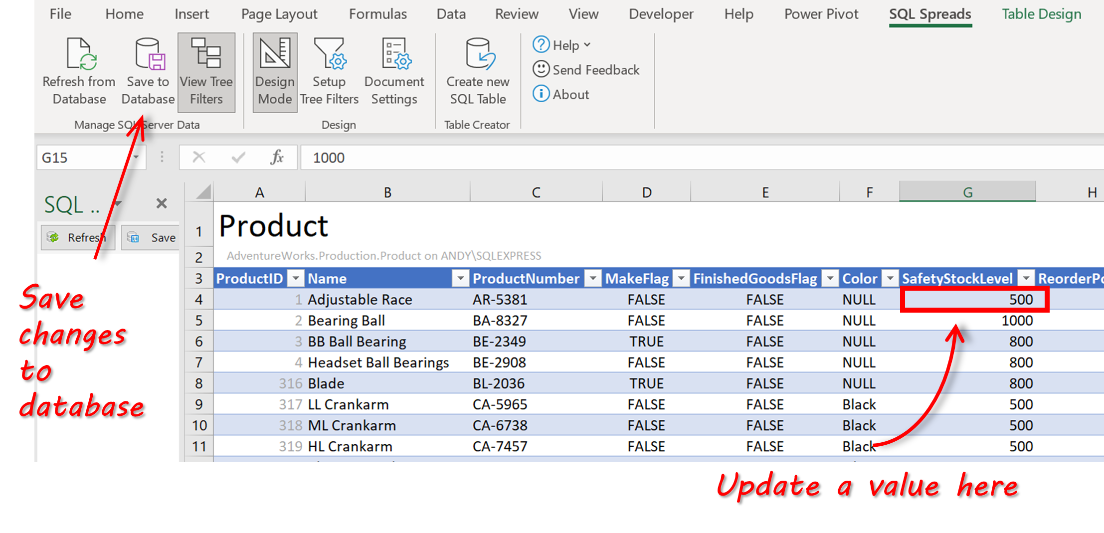
You can also update the prices in the product table directly in Excel, and save the changes back to SQL Server. To do this you simply make the edits in the table in Excel and then click on the ‘Save to Database’ button to get the changes written to the table in SQL Server.
There are some other ways to import an Excel file to a table in SQL Server. Here are some of the other methods.
- SQL Server Import Wizard – a wizard-based import tool inside SQL Server Management Studio. Ideal for one-time imports when you have an Excel document that you need to import into a table in SQL Server. The pros include flexibility and lots of settings to finetune the import. The biggest drawback is that you need to run through a dozen Wizard dialogs with lots of settings each time you need to import the data. More info about the SQL Server Import Wizard is available here .
- SSIS – this is the oil tanker for moving data between different sources. You can do almost any task you like, but you will need to put in lots of time to get started, and it will take still more time to maintain and change the solution down the line. The pros include good versatility and plenty of available features; the main con is the time you will have to put in to learn the tool. More info about SSIS is available here .
- The BCP utility – a command line-based tool that offers a huge number of settings – if you are a coder, this is the tool to use. More info about the BCP utility is available here .
Summary – insert data from Excel to SQL Server
In this article, we’ve looked at 2 easy ways to insert data from Excel to SQL Server.
If you know how to use SQL Server Management Studio, the copy and paste feature is a great option when you need to quickly and easily import data from Excel to SQL Server. The process is simple and doesn’t require any special knowledge or tools, and can be used in tables with up to a few tens of thousands of rows of data. It can also cater for scenarios such as tables with an auto-incrementing identity key, or if you need to connect to SQL Server on a remote machine using a Remote Desktop Connection.
If you don’t have access to SQL Server Management Studio, you can use the SQL Spreads Excel Add-In to insert data from Excel to SQL. It’s quick and easy to use for non-technical users. For more advanced users, there are some cool features such as lookup columns, pivot options, and data validation which allow you to create robust data management solutions.
Download your free trial of SQL Spreads and get in touch with us if you have any questions.

Johannes Åkesson
Worked in the Business Intelligence industry for the last 15+ years.
Founder of SQL Spreads – the data management
solution to import, update and manage
SQL Server data from within Excel.
Источник
A table in Excel is a complex array with set of parameters. It can consist of values, text cells, formulas and be formatted in various ways (cells can have a certain alignment, color, text direction, special notes, etc.).
When you copy a table, sometimes you do not have to transfer all of its elements, but only some of its. Consider how this can be done.
The past special
It is very convenient to carry out the transfer of the data in the table using the past special. It allows you to select only those parameters that we need when copying. Let’s consider an example.
We have the table with the indicators for the presence of macaroni of certain brands in the warehouse of the store. It is clearly visible, how many kilograms were at the beginning of the month, how much of them were bought and sold, and also the balance at the end of the month. Two important columns are highlighted in different colors. The balance at the end of the month is calculated by the elementary formula.
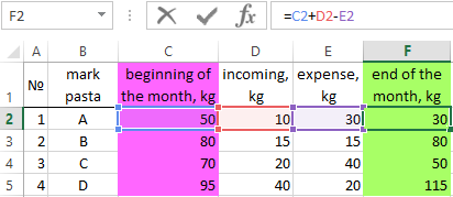
We will try to use the PAST SPECIAL command and copy all the data.
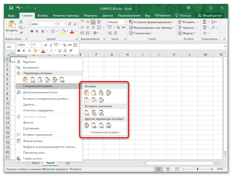
First we select the existing table, right click the menu and click on COPY.
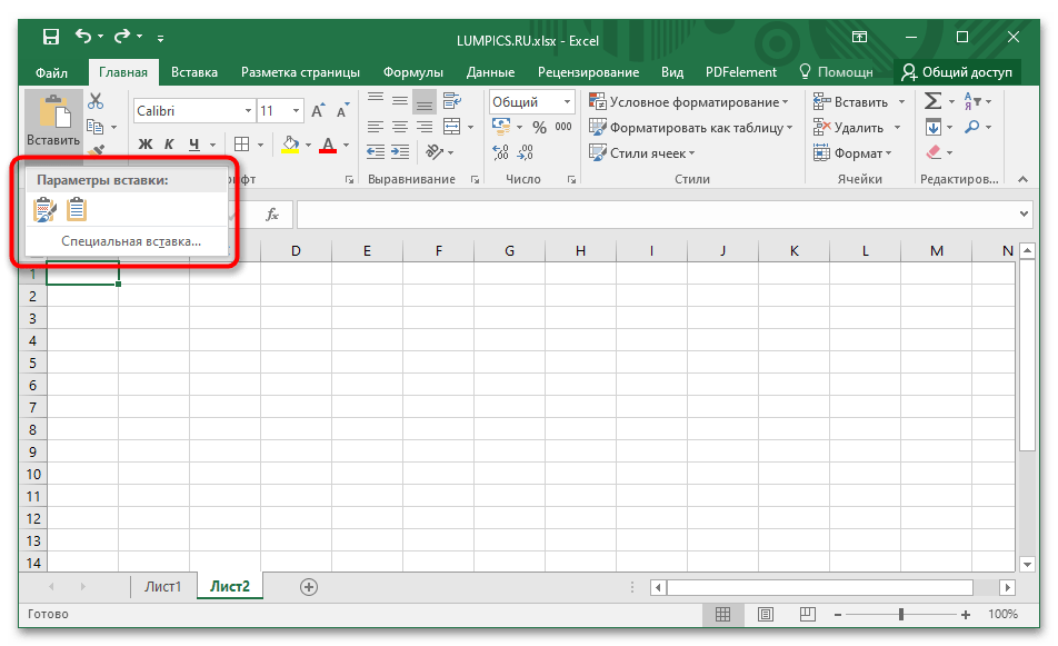
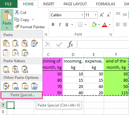
In the free cell, we call the menu again with the right button and press the PAST SPECIAL.
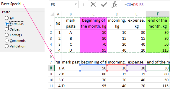
If we leave everything as is by default and just click OK, the table will be inserted completely, with all its parameters.
Let’s try to experiment. In the PAST SPECIAL we choose another item, for example, FORMULAS. We have already received an unformatted table, but with working formulas.
Now we will insert not the formulas, but only the VALUES of the results of calculations.
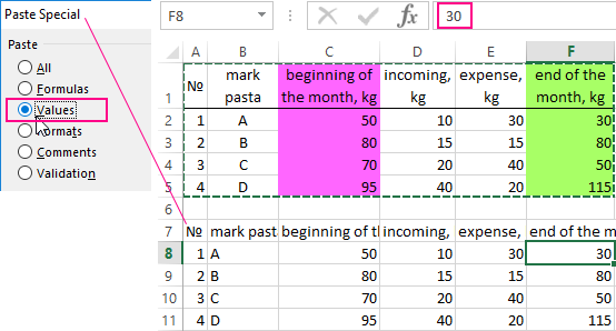
That a new table with values to get the appearance similar to the sample, you need to select it and insert the FORMATS using a special insert.
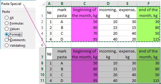
Now let’s try to choose the item WITHOUT FRAME. We got the full table, but only without the allocated borders.
The wholesome advice! To migrate the format along with the size of the columns, you need to select not the range of the source table, but the entire columns (in this case, the A: F range) before the copying.
Similarly, you can experiment with each item of the PAST SPECIAL to see clearly how it works.
Transfer of data to another sheet
Transferring data to other worksheets in the Excel workbook allows you to link multiple tables. This is convenient because when you replace a value on one sheet, the values change on all the others. When creating annual reports, this is an indispensable thing.
Consider how this works. For a start we rename Excel sheets in months. Then, with the helping of the PAST SPECIAL that we already know, we move the table to February and remove the values from the three columns:
- At the beginning of the month.
- The incoming.
- The expense.
The column «At the end of the month» is given by the formula, so when you delete values from the previous columns, it is automatically reset to zero.
We will transfer to the data on the remainder of macaroni of each brand from January to February. This is done in a couple of clicks.
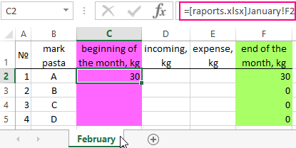
- On the FEBRUARY sheet we place the cursor in the cell, indicating the amount of macaroni of grade A at the beginning of the month. You can see the picture above — this will be cell D3.
- We put in this cell to the sign EQUAL.
- Go to the JANUARY sheet and click on the cell showing the amount of macaroni of grade A at the end of the month (in this case it is cell F2).
We get the following: in the cell C2 the formula was formed, which sends us to the cell F2 of the JANUARY sheet. Stretch the formula down to know the amount of macaroni of each brand at the beginning of February.
Similarly, you can transfer the data to all months and get to the visual annual report.
Data transfer to another file
Similarly, you can transfer data from one file to another one. This book in our example is called EXCEL. Create another one and name it EXAMPLE.
Note. You can create new Excel files even in different folders. The program will automatically search for the specified book, regardless of which folder and on what drive of the computer it is located.
We copy in the book EXAMPLE to the table using the same PAST SPECIAL and again delete the values from the three columns. We will perform the same actions as in the previous paragraph, but we will not go to another sheet, but to another book only.
We have received to the new formula, which shows that the cell refers to the book EXCEL. And we see that the cell =[raports.xlsx]January!F2 looks like =[raports.xlsx]January!$F$2, i. e. it is fixed. And if we want to stretch to the formula in other brands of macaroni, first you need to remove the dollar badges for removing to the commit.
Now you know how to correctly transfer data from tables within one sheet, from one sheet to another, and from one file to another one.
When working in Excel, it is not definite that data will be in a single worksheet. It can be in multiple worksheets on multiple tables. If we want to merge tables, there are various methods to do that so that we can have data in a single table. It is known as merging tables in Excel. We can do this by using the VLOOKUP or INDEX and MATCH functions.
While analyzing the data, we might gather all the necessary information in a single worksheet. Unfortunately, it is a common problem when data is divided across many worksheets or workbooks. There are many ways to merge the data from multiple tables into one table in excelIn excel, tables are a range with data in rows and columns, and they expand when new data is inserted in the range in any new row or column in the table. To use a table, click on the table and select the data range.read more.
Table of contents
- Merge Tables in Excel
- How to Merge 2 Tables in Excel?
- Sheet 1: Table 1: CustomerInfo
- Sheet 2: Table 2: ProductDetails
- Things to Remember About Merge 2 Tables in Excel
- Recommended Articles
- How to Merge 2 Tables in Excel?
You can download this Merge Table Excel Template here – Merge Table Excel Template
How to Merge 2 Tables in Excel?
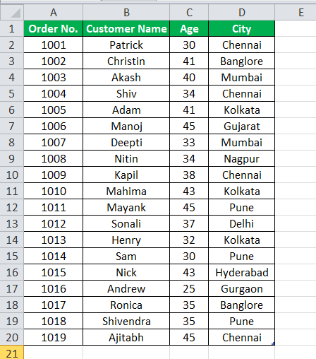
We have given customer data city-wise in two tables. We have taken 20 records.
Sheet 1: Table 1: CustomerInfo
Sheet 2: Table 2: ProductDetails
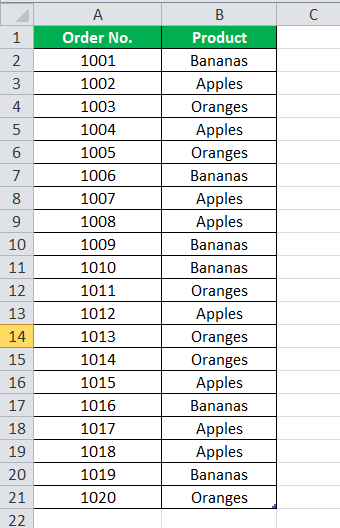
In both the tables, “Order No.” is the common information on which basis we will create a relationship between them.
Below are the steps for merging these two tables:
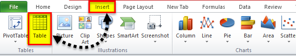
- Click on any cell in the “Customer Info” table. Go to the “INSERT” tab and click on the “Table” option under the “Tables” section. You may refer to the below screenshot.

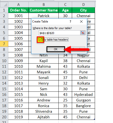
- Then, the “Create Table” dialog box will appear. Our table “CustomerInfo” has column headers. Hence, the checkbox “My table has headers” should be checked. Refer to the below screenshot.

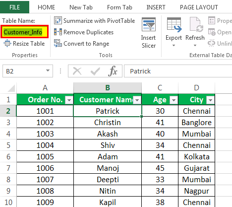
- It will convert our data into a table format. Now, click on the “Table Name” field under the “Properties” section and give the name of this table as “Customer_Info.”

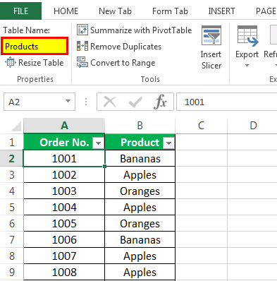
- Follow the same steps for another table, “ProductDetails.” We have given the name “Products” to another table. Refer to the below screenshot.
- Click on somewhere on the “Customer_Info” table then, Then go to the “Insert” tab, and click on the “PivotTable” option under the “Tables” section.
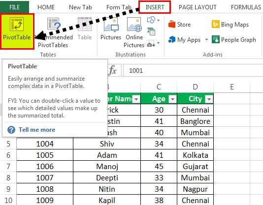
- A dialog box for “Create PivotTable” will appear. Next, tick the checkbox “Add this data to the Data Model,” as shown in the below screenshot.
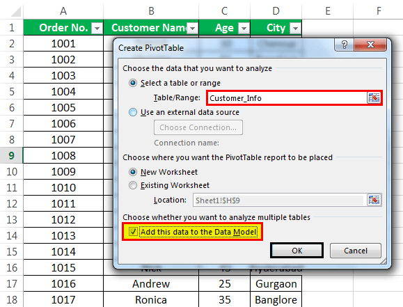
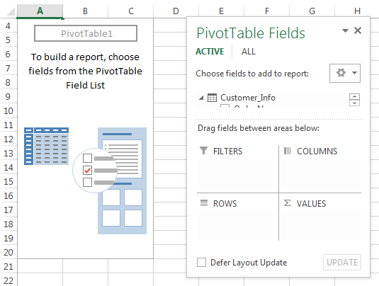
- Click on “OK.” Then, it will open a new sheet with a new Pivot Table FieldsPivot table calculated fields are formulas with reference to other fields, and calculated values refer to other values within a specific pivot field.read more section on the right side, as shown in the below screenshot.
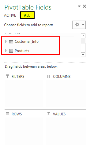
- Click on the “ALL” tab in the “PivotTable Fields” section. It will display all the tables created by us. Refer to the below screenshot.
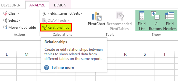
- Now, click on the “Relationships” option under the “Calculations” section, as shown in the below screenshot.
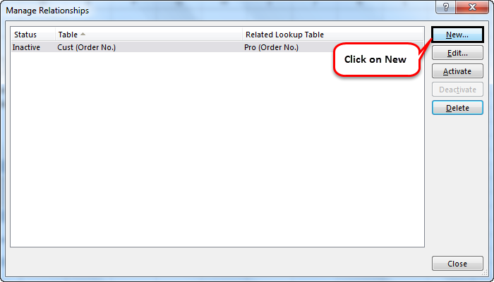
- It will open a dialog box for creating a relationship between these tables. First, click on the “New” button. Then, refer to the below screenshot.
- Again, it will open a dialog box as shown below, and created tables are listed here.
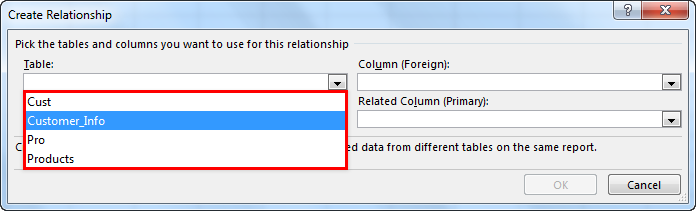
- As there is one field, “Order No.” is common in both tables. Hence we will create a relationship between these tables using this common field/column.
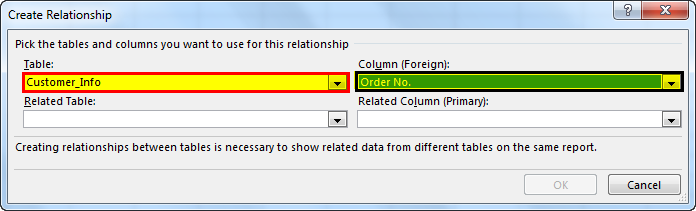
- Select “Customer_Info” under the “Table” section and the “Order No.” field under the “Column (Foreign)” section. Then, refer to the below screenshot.
- Select another table, “Products,” under the “Related Table” section and select the “Order No.” field under the “Related Column” section. Then, refer to the below screenshot.
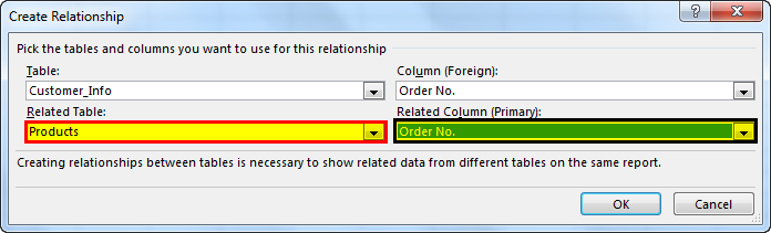
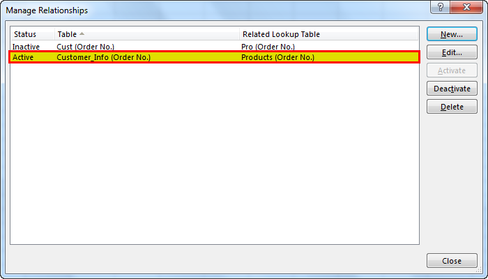
- The primary key is the unique values that appear once in the table. Then, click on “OK.” It will display the relationship, as shown in the below screenshot.
- Now, we can drag and drop the field accordingly to see the result. Next, click on the “Customer_Info” table, as shown in the below screenshot.
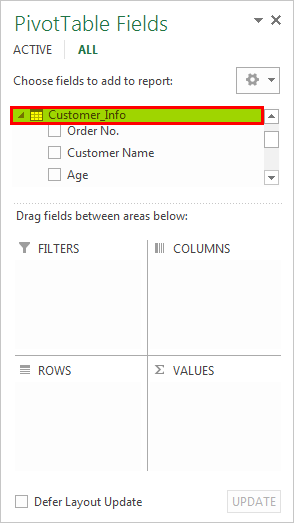
- Under the “ROWS” box, drag fields “Order No.”, “Customer Name,” and the “City.”
- Drag the “Age” field under the “FILTERS” box.
- Drag the “Product” field under the “COLUMNS” box, and the “VALUES” box for the products count.

The final result is below:
Accordingly, as per the requirement, we can drag and drop the fields.

Things to Remember About Merge 2 Tables in Excel
- We can merge more than two tables using this process.
- There should be one column common in each table.
- That one common column will work as a primary key in this process. Hence, this field should have unique values.
Recommended Articles
This article is a guide to Merge Tables in Excel. We discuss merging two tables in Excel by matching a column with practical examples and a downloadable Excel template. You may learn more about Excel from the following articles: –
- Excel Data ModelA data model in Excel is a data table in which two or more tables are linked together by a common or many data series. Data from several sheets is combined to create a unique table in data model tables.read more
- Create a Pivot Chart in Excel
- Use Pivot Table Slicer
- Excel Table StylesExcel comes with a number of table styles that you may quickly apply to a table format. In Excel, you can design and use a new custom table style of your choice. read more
Reader Interactions
Bottom Line: Learn helpful tips and keyboard shortcuts to insert and format Excel tables quickly.
Skill Level: Beginner
Video Tutorial
Download the Excel File
The file I use in the video can be downloaded here:
Creating Tables in Excel
There are two quick and easy ways to insert an Excel Table using existing data in a spreadsheet.
1. Using the Insert Tab
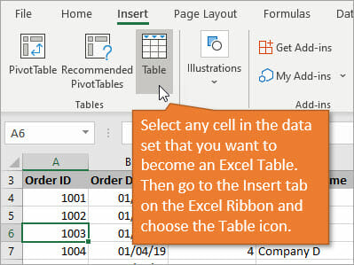
The first way is to go to the Insert tab in the Ribbon and select the Table icon. (First make sure your selected cell is anywhere in the data set that you want to convert into a table). The keyboard shortcut for this procedure is Ctrl + T.
This will bring up the Create Table box, which is prepopulated with the existing boundaries of the data set you’re in. Assuming you want all of that data in your table, just select OK.
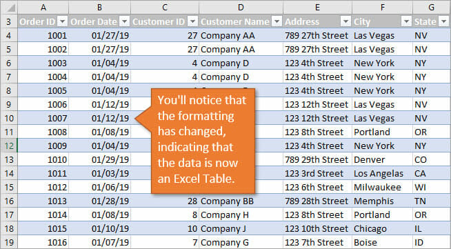
Your data field has now been converted to an Excel Table, which makes it easier to sort, filter, and format the data.
Changing the Style
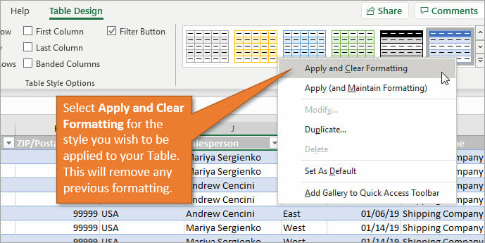
If you had applied formatting to your data before making it a table, the Insert Table feature does not override that formatting. If you want to change the style, you can go to the Table Design tab on the Ribbon and right-click on the selected style. This gives you an option to Apply and Clear Formatting. When you select that option, the previous formatting is replaced with the style you’ve selected.
2. Using the Home Tab
Another way to insert a table, which might be a little bit faster if you have formatting that you want to clear, is using the Home tab.
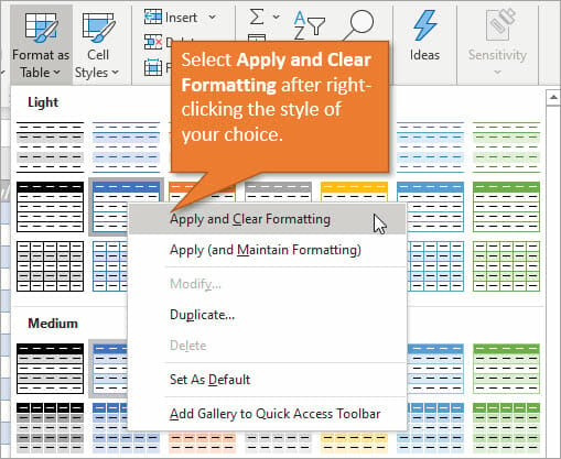
From the Home tab on the Ribbon, select the Format as Table menu. This will bring up a gallery of different styles to choose from. If, as above, you right-click on the style you want, and select Clear and Apply Formatting, you’ve combined the creating of the table with the formatting at the same time.
Keyboard Shortcuts for This Method
The keyboard shortcut to open the Format as Table menu is Alt, H, T. Then you can use the arrow keys to select the style you want and hit Enter.
This does not clear the existing formatting, but if you want to do that, you can use the keyboard shortcut above. But once you’ve highlighted the style you want, click on the Menu key to bring up the right-click menu that we’ve already seen, then press C for the Apply and Clear Formatting option. The underlined letter is the shortcut key for each option.
So the full keyboard shortcut to create a Table and Clear and Apply Formatting is: Alt, H, T, Menu, C, Enter
If you’re not sure what the Menu key looks like, or want to know more about how to use it, I’ve created these helpful posts:
Excel Keyboard Shortcuts for the Menu Key
Best Keyboards for Excel Keyboard Shortcuts
Duplicating a Style
If you always want to use the same style within a workbook, here’s a tip to quickly access the style you like. From the gallery of styles, right-click on the one you like and choose Duplicate.
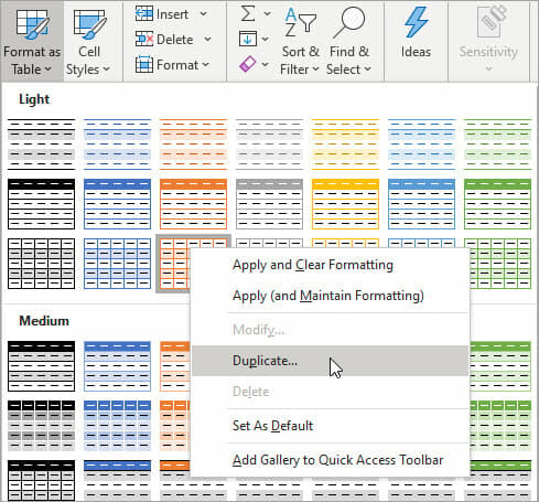
This will open a box allowing you to customize the style or leave it as is. Once you kit OK, this style will appear at the top of your gallery as a Custom style.
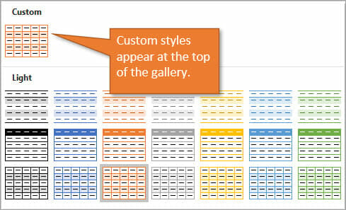
This placement at the top simply helps save time hunting for the style you want each time you create a new table. The Alt, H, T, Enter keyboard shortcut will also apply this first style in the Custom section.
You can also follow that with the Menu, C shortcut to Clear and Apply Formatting.
Keep in mind that this custom styling is only for the workbook you are in and does not carry over to other workbooks.
Related Posts
If you are new to Excel Tables, you can learn more about them here: Excel Tables Tutorial Video – Beginners Guide for Windows & Mac
When naming your tables, it’s best to use a prefix. This tutorial explains why: Best Practices for Naming Tables
And this video will help you when you are creating pivot tables: 5 Reasons to Use an Excel Table as the Source of a Pivot Table
Conclusion
Excel Tables are a great way to work with data. I hope this post is helpful as you create them in your spreadsheets. If you have questions or tips about working with tables, I’d love to hear them in the comments.
In this post, we’re going to learn everything there is to know about Excel Tables!
Yes, I mean everything and there’s a lot.
This post will tell you about all the awesome features Excel Tables have and why you should start using them.
What is an Excel Table?
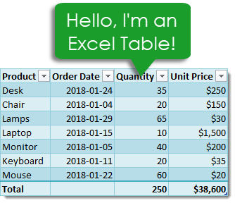
Excel Tables are containers for your data.
Imagine a house without any closets or cupboards to store your things, it would be chaos! Excel tables are like closets and cupboards for your data, they help to contain and organize data in your spreadsheets.
In your house, you might put all your plates into one kitchen cupboard. Similarly, you might put all your customer data into one Excel table.
Tables tell excel that all the data is related. Without a table, the only thing relating the data is proximity to each other.
Ok, so what’s so great about Excel Tables other than being a container to organize data? A lot actually. This post will tell you about all the awesome features tables have and should convince you to start using them.
Video Tutorial
The Parts of a Table
Throughout this post, I’ll be referring to various parts of a table, so it’s probably a good idea that we’re both talking about the same thing.
This is the Column Header Row. It is the first row in a table and contains the column headings that identify each column of data. Column headings must be unique in the table, they cannot be blank and they cannot contain formulas.
This is the Body of the table. The body is where all the data and formulas live.
This is a Row in the table. The body of a table can contain one or more rows and if you try to delete all the rows in a table a single blank row will remain.
This is a Column in the table. A table must contain at least one column.
This is the Total Row of the table. By default, tables don’t include a total row but this feature can be enabled if desired. If it’s enabled, it will be the last row of the table. This row can contain text, formula or remain blank. Each cell in the total row will have a drop down menu that allows selection of various summary formula.
Create a Table from the Ribbon
Creating an Excel Table is really easy. Select any cell inside your data and Excel will guess the range of your data when creating the table. You’ll be able to confirm this range later on. Instead of letting Excel guess the range you can also select the entire range of data in this step.
With the active cell inside your data range, go to the Insert tab in the ribbon and press the Table button found in the Tables section.
The Create Table dialog box will pop up. Excel guesses the range and you can adjust this range if needed using the range selector icon on the right hand side of the Where is the data for your table? input field. You can also adjust this range by manually typing over the range in the input field.
Checking the My table has headers box will tell Excel the first row of data contains the column headers in your table. If this is unchecked Excel will create generic column headers for the table labelled Column 1, Column 2 etc…
Press the Ok button when you’re satisfied with the data range and table headers check box.
Congratulations! You now have an Excel table and your data should look something like the above depending on the default style of your tables.
Contextual Table Tools Design Tab
Whenever you select a cell inside a table, you will notice a new tab appear in the ribbon labelled Table Tools Design. This is a contextual tab and only appears when a table is selected. When the active cell moves outside the table, the tab will disappear again.
This is where all the commands and options related to tables will live. This is where you’ll be able to name your table, find table related tools, enable or disable table elements and change your table’s style.
Create a Table with a Keyboard Shortcut
You can also create a table using a keyboard shortcut. The process is the same as described above but instead of using the Table button in the ribbon you can press Ctrl + T on your keyboard. It’s easy to remember since T is for Table!
There is actually another keyboard shortcut that you can use to create tables, Ctrl + L will also do the same thing. This is a legacy from when tables were called lists (L is for List).
Name a Table
Anytime you create a new table Excel will give it an initial generic name starting with Table1 and increasing sequentially. You should always rename your table with a descriptive and short name.
Not all names are allowed. There are a few rules for a table name.
- Each table must have a unique name within a workbook.
- You can only use letters, numbers and the underscore character in a table name. No spaces or other special characters are allowed.
- A table name must begin with either a letter or an underscore, it can not begin with a number.
- A table name can have a maximum of 255 characters.
Select any cell inside your table and the contextual Table Tools Design tab will appear in the ribbon. Inside this tab you can find the Table Name under the Properties section. Type over the generic name with your new name and press the Enter button when finished to confirm the new name.
Rename a Table
Renaming a table you’ve already named is the same process as naming a table for the first time. If you think about it, when you first name a table you’re actually renaming it from the generic name of Table1 to a new name.
So go back to the Table Tools Design tab and type your new name over the old one in the Table Name and press Enter. Easy, and the name is changed.
Changing your table name this way requires navigating to your table and selecting a cell within it, so it can be tedious if you need to rename a lot of tables across different sheets in your workbook. Instead, you can change any of your table names without going to each table using the Name Manager.
Go to the Formula tab and press the Name Manager button in the Defined Names section. You’ll be able to see all your named objects here. The table objects will have a small table icon to the left of the name. You can filter to show only the table objects using the Filter button in the upper right hand corner and selecting Table Names from the options.
You can then edit any name by selecting the item and pressing the Edit button. You’ll be able to change the name and add some comments to describe the data in your table.
Navigate Tables with the Name Box
You can easily navigate to any table in your workbook using the name box the the left of the formula bar. Click on the small arrow on the right side of the name box and you will see all table names in the workbook listed. Click on any of the tables listed and you will be taken to that table.
Convert a Table Back to a Normal Range
Ok, you changed your mind and don’t want your data inside a table anymore. How do you convert it back into a regular range?
If changing it to a table was the last thing you did, Ctrl + Z to undo your last action is probably the quickest way.
If it wasn’t the last thing you did, then you’re going to need to use the Convert to Range command found in the Table Tools Design tab under the Tools section.
You’ll be prompted to confirm that you really want to convert the table to a normal range. Noooooo, don’t do it, tables are awesome!
If you click on yes, then all the awesome benefits from tables will be gone except for the formatting design. You’ll need to manually clear this from the range if you want to get rid it. You can do this by going to the Home tab then pressing the Clear button found in the Editing section, then selecting Clear Formats.
This can also be done from the right click menu. Right click anywhere in the table and select Table from the menu and then Convert to Range.
Select the Entire Column
If your data is not inside a table then selecting an entire column of the data can be difficult. The usual way would be to select the first cell in the column and then hold Ctrl + Shift then press the Down arrow key. If the column has blank cells, then you might need to press the Down arrow key a few times until you reach the end of the data.
The other option is to select the first cell and then use the scroll bar to scroll to the end of your data then hold the Shift key while you select the last column.
Both options can be tedious if you have a lot of data or there are a lot of blanks cells in the data.
With a table, you can easily select the entire column regardless of blank cells. Hover the mouse cursor over the column heading until it turns into a small arrow pointing down then left click and the entire column will be selected. Left click a second time to include the column heading and any total row in the selection.
Another way to quickly select the entire column is to place the active cell cursor on any cell in the column and press Ctrl + Space. This will select the entire column excluding the column header and total row. Press Ctrl + Space again to include the column headers and total row.
Select the Entire Row
Selecting the entire row is just as easy. Hover the mouse cursor over the left side of the row until it turns into a small arrow pointing left then left click and the entire row will be selected. This works on both the column heading row and total row.
Another way to quickly select the entire row is to place the active cell cursor on any cell in the row and press Shift + Space.
Select the Entire Table
It’s also possible to select the entire table and there are a couple different ways to do this.
You can place the active cell cursor inside the table and press Ctrl + A. This will select the entire body of the table excluding the column headers and total row. Press Ctrl + A again to include the column headers and total row.
Hover the mouse over the top left hand corner of the table until the cursor turns into a small black diagonal right and downward pointing arrow. Left click once to select only the body. Left click a second time to include the header row and total row.
You can also select the table with the mouse. Place the active cell inside the table and then hover the mouse cursor over any edge of the table until it turns into a four way directional arrow then left click. This will also select the column headers and total row.
Select Parts of the Table from the Right Click Menu
You can also select rows, columns or the entire table using the right click menu. Right click anywhere on the row or column you want to select then choose Select and pick from the three options available.
Add a Total Row
You can add a total row which allows you to display summary calculations in the last row of your table.
Adding summary calculations at the bottom of your data can be dangerous as they might end up getting included by accident in a pivot table using the data. This is another advantage of tables, as the total row won’t be included in any pivot tables created with the table.
To enable the total row, go to the Table Tools Design tab and check the Total Row box found in the Table Style Options section.
You can temporarily disable the total row without losing the formulas you added to it. Excel will remember the formulas you had and they will appear when you enable it again.
Each cell in the total row has a drop down menu that allows you to pick various aggregating functions to summarize the column of data above.
You can also enter your own formulas. I’ve entered a SUMPRODUCT formula in the Unit Price total to sum the Quantity x Unit Price to calculate a total sale amount. Formulas don’t have to return a number, they can also be text results.
Constant numerical or text values are also allowed anywhere in the total row. In fact the leftmost column will usually contain the text Total by default.
Add a Total Row with a Right Click
You can also add the total row with a right click. Right click anywhere on the table and the choose Table and Total Row from the menu.
Add a Total Row with a Keyboard Shortcut
Another way to quickly add the total row is to place the active cell cursor inside your table and use the Ctrl + Shift + T keyboard shortcut.
Disable the Column Header Row
The column header row is enabled by default, but you can disable it. This doesn’t delete the column headers, it’s essentially like hiding them as you will still reference columns based on the column header name.
Go to the Table Tools Design tab and uncheck the Total Row box found in the Table Style Options section.
Add Bold Format to the First or Last Columns
You can enable a bold formatting on either your first or last column to highlight it and draw attention to them over other columns.
Go to the Table Tools Design tab and check either of the First Column or Last Column boxes (or both) found in the Table Style Options section.
Add Banded Rows or Columns
Banded rows are already enabled by default, but you can turn them off if you want. Banded columns are disabled by default, so you need to enable them if you want them.
To enable or disable either, go to the Table Tools Design tab and check or uncheck the Banded Rows or Banded Columns boxes found in the Table Style Options section.
I generally find banded rows are the most useful and if you enable banded columns at the same time, the table starts to look a little messy. I recommend one or the other and not both at the same time.
- Table with no banded rows or columns.
- Table with banded rows only.
- Table with banded columns only.
- Table with both banded rows and columns.
Table Filters
By default, the table filters option is enabled. You can disable them from the Table Tools Design tab by unchecking the Filter Button box found in the Table Style Options section.
You can also toggle the filters on or off from the active table by using the regular filter keyboard shortcut of Ctrl + Shift + L.
If you left click on any of the filters, it will bring up the familiar filter menu where you can sort your table and apply various filters depending on the type of data in the column.
The great thing about table filters is you can have them on multiple tables in the same sheet simultaneously. You will need to be careful though as filtered items in one table will affect the other tables if they share common rows. You can only have one set of filters at a time in a sheet of data without tables.
Total Row with Filters Applied
When you select a summary function from the drop down menu in the total row, Excel will create the corresponding SUBTOTAL formula. This SUBTOTAL formula ignores hidden and filtered items. So when you filter your table these summaries will update accordingly to exclude the filtered values.
Note that the SUMPRODUCT formula in the Unit Price column still includes all the filtered values while the SUBTOTAL sum formula in the Quantity column does not.
Column Headers Remain Visible When Scrolling
If you scroll down while the active cell is in a table, its column headers will remain visible along with the filter buttons. The table’s column headings will get promoted into the sheet’s column headings where we would normally see the alphabetic column name.
This is extremely handy when dealing with long tables as you won’t need to scroll back up to the top to see the column name or use the filters.
Automatically Include New Rows and Columns
If you type or copy and paste new data into the cells directly below a table, they will automatically be absorbed into the table.
The same thing happens when you type or copy and paste into the cells directly to the right of a table.
Automatically Fill Formulas Down the Entire Column
When you enter a formula inside a table it will automatically fill the formula down the entire column.
Even when a formula has already been entered and you add new data to the row directly below the table any existing formulas will automatically fill.
Editing an existing formula in any of the cells will also update the formula in the entire column. You’ll never forget to copy and paste down a formula again!
Turn Off the Auto Include and Auto Fill Settings
You can turn off the feature that automatically adds new rows or columns and fills down formulas.
Go to the File tab and select Options. Choose Proofing then press the AutoCorrect Options button. Navigate to the AutoFormat As You Type tab in the AutoCorrect dialog box.
Unchecking the Include new rows and columns in table option allows you to type directly underneath or to the right of a table without it absorbing the cells.
Unchecking the Fill formulas in tables to create calculated columns option means the formulas in a table will no longer automatically fill down the column.
Resize with the Handle
Every table comes with a Size Handle found in the bottom rightmost cell of the table.
When you hover the mouse over the handle, the cursor will turn into a double-sided diagonally slanting arrow and you can then click and drag to resize the table. You can either expand or contract the size. Data will be absorbed into the table or removed from it accordingly.
Resize with the Ribbon
You can also resize the table from the ribbon. Go to the Table Tools Design tab and press the Resize Table command in the Properties section.
The Resize Table dialog box will pop up and you’ll be able to select a new range for your table. Use the range selector icon to select a new range. You can select either a larger or smaller range, but The table headers will need to remain in the same row and the new table range must overlap the old table range.
Add a New Row with the Tab Key
You can add a new blank row to a table with the Tab key. Place the active cell cursor inside the table on the cell containing the sizing handle and press the Tab key.
The tab key act like a carriage return and the active cell is taken to the rightmost cell on a new line that’s added directly below.
This is a handy shortcut to know because when the total row is enabled, it’s not possible to add a new row by typing or copying and pasting data directly below the table.
Insert Rows or Columns
You can insert extra rows or columns into a table with a right click. Select a range in the table and right click then choose Insert from the menu. You can then either choose to insert Table Columns to the Left or Table Rows Above.
Table Columns to the Left will insert the number of columns selected to the left of the selection and the number of rows in the selection is ignored.
Table Rows Above will insert the number of rows selected just above the selection and the number of columns in the selection is ignored.
Delete Rows or Columns
Deleting rows or columns has a similar story to inserting them. Select a range in the table and right click then choose Delete from the menu. You can then either choose to delete Table Columns or Table Rows.
Formats in a Table Automatically Apply to New Rows
When you add new data to your table, you don’t need to worry about applying formatting to match the rest of the data above. Formatting will automatically fill down from above if the formatting has been applied to the entire column.
I’m not just talking about the table style formats. Other formatting like dates, numbers, fonts, alignments, borders, conditional formatting, cell colours etc. will all automatically fill down if they’ve been applied to the whole column.
If you’ve formatted all your numbers as a currency in a column and you add new data, it too will get the currency format applied to it.
You never need to worry about inconsistent formatting in your data.
Add a Slicer
You can add a slicer (or several) to a table for an easy to use filter and visual way to see what items the table is filtered on.
Go to the Table Tools Design tab and press the Insert Slicer button found in the Tools section.
Change the Style
Changing the styling of a table is quick and easy. Go to the Table Tools Design select a new style from the selection found in the Table Styles section. If you left click the small downward arrow on the right hand side of the styles palette, it will expand to show all available options.
These table styles apply to the whole table and will also apply to any new rows or columns added later on.
There are many options to choose from including light, medium and dark themes. As you hover over the various selections, you’ll be able to see a live preview in the worksheet. The style won’t actually change until you click on one though.
You can even create your own New Table Style.
Set a Default Table Style
You can set any of the styles available as the default so that when you create a new table you don’t need to change the style. Right click on the style you want to set as the default and then choose Set As Default from the menu.
Unfortunately, this is a workbook level setting and will only affect the current workbook. You will need to set the default for each workbook you create if you don’t want the application default option.
Only Print the Selected Table
When you place the active cell cursor inside a table and then try to print, there is an option to only print the selected table. Go to the Print menu screen by either going to the File tab and selecting Print or using the Ctrl + P keyboard shortcut, then select Print Selected Table in the settings.
This will remove any items from the print area that are not in the table.
Structured Referencing
Tables come with a useful feature called structured referencing which helps to make range references more readable. Ranges within a table can be referred to using a combination of the table name and column headings.
Instead of seeing a formula like this =SUM(D3:D9) you might see something like this =SUM(Sales[Quantity]) which is much easier to understand the meaning of.
This is why naming your table with a short descriptive name and column headings is important as it will improve the readability of the structured references!
When you reference specific parts of a table, Excel will create the reference for you so you don’t need to memorize the reference structure but it will help to understand it a bit.
Structured references can contain up to three parts.
- This is the table name. When referencing a range from inside the table this part of the reference is not required.
- These are range identifiers and identify certain parts of the reference for a table like the headers or total row.
- These are the column names and will either be a single column or a range of columns separated by a full colon.
Example of structured References for a Row
=Sales[@[Unit Price]]will reference a single cell in the body.=Sales[@[Product]:[Unit Price]]will reference part of the row from the Product column to the Unit Price column including all columns in between.=Sales[@]will reference the full row.
Example of Structured References for Columns
=Sales[Unit Price]will reference a single column and only include the body.=Sales[[#Headers],[#Data],[Unit Price]]will reference a single column and include the column header and body.=Sales[[#Data],[#Totals],[Unit Price]]will reference a single column and include the body and total row.=Sales[[#All],[Unit Price]]will reference a single column and include the column header, body and total row.
Example of Structured References for the Total Row
=Sales[#Totals]will reference the entire total row.=Sales[[#Totals],[Unit Price]]will reference a cell in the total row.=Sales[[#Totals],[Product]:[Unit Price]]will reference part of the total row from the Product column to the Unit Price column including all columns in between.
Example of Structured References for the Column Header Row
=Sales[#Headers]will reference the entire column header row.=Sales[[#Headers],[Order Date]]will reference a cell in the column header row.=Sales[[#Headers],[Product]:[Unit Price]]will reference part of the column header row from the Product column to the Unit Price column including all columns in between.
Example of Structured References for the Table Body
=Saleswill reference the entire body.=Sales[[#Headers],[#Data]]will reference the entire column header row and body.=Sales[[#Data],[#Totals]]will reference the entire body and total row.=Sales[#All]will reference the entire column header row, body and total row.
Using Intellisense
One of the great things about a table is the structured references will appear in Intellisense menus when writing formulas. This means you can easily write a formula using the structured references without remembering all the fields in your table.
After typing the first letter of the table name, the IntelliSense menu will show the table name among all the other objects starting with that letter. You can use the arrow keys to navigate to it and then press the Tab key to autocomplete the table name in your formula.
If you want to reference a part of the table, you can then type a [ to bring up all the available items in the table. Again, you can navigate with the arrow keys and then use the Tab key to autocomplete the field name. Then you can close the item with a ].
Turn Off Structured Referencing
If you’re not a fan of being forced to use the structured referencing system, then you can turn it off. Any formulas that have been entered using the structured referencing will remain and they will still work the same. You’ll also still be able to use structured references, Excel just won’t automatically create them for you.
To turn it off, go to the File tab and then select Options. Choose Formulas on the side pane and then uncheck the Use table names in formulas box and press the Ok button.
Summarize with a PivotTable
You can create a pivot table from your table in Table Tools Design tab, press the Summarize with PivotTable button found in the Tools section. This will bring up the Create PivotTable window and you can create a pivot table as usual.
This is the same as creating a pivot table from the Insert tab and doesn’t give any extra options specific to tables.
Remove Duplicates from a Table
You can create remove duplicate rows of data from your table in Table Tools Design tab, press the Remove Duplicates button found in the Tools section. This will bring up the Remove Duplicates window and delete duplicate values for one or more columns in the table.
This is the same as removing duplicates from the Data tab and doesn’t give any extra options specific to tables.
About the Author
John is a Microsoft MVP and qualified actuary with over 15 years of experience. He has worked in a variety of industries, including insurance, ad tech, and most recently Power Platform consulting. He is a keen problem solver and has a passion for using technology to make businesses more efficient.
Today I want to show off a quick trick I learned many years ago that is useful to this day.
The Scenario: you have a spreadsheet, CSV file, or some other delimited flat file and need to load that into a database. There are many options to load data into SQL Server; however, a quick method I am fond of is to use Microsoft Excel and manipulate the data to craft insert statements then paste into SSMS and execute.
Read on to see how to parse and load a CSV flat file, character delimited flat file, and columnar text.

Many beginning and aspiring database people start work not as a developer or admin but as an analyst. It is common to work with large data sets and receive an Excel workbook that needs to be imported into your SQL Server database.
In the below examples I will be using the AdventureWorks2016 database to demonstrate. Let’s use the Person.Address table. I will stage a small sample of data to demo by creating a smaller subset of just NC residents.
select * from Person.[Address] where City = 'Raleigh'; --let's pick a good city...
select * from Person.[Address] where StateProvinceID = 42; --8 expanded to a nice state (NC)
select * into Address_NC from Person.[Address] where StateProvinceID = 42;
select * from Address_NC; --8
Here are the contents of the table:

Let us also capture the table definition. This can be important for dealing with constraints, indexes, defaults, and identity columns.

Protip: alt + F1 is a default keyboard shortcut in SSMS to calling sp_help on the table.
There is an identity column so we will take that into account when crafting our insert statements
CSV Flat File
Assume: you are given a CSV flat file and need to quickly load it into a database – no 3rd party tools. Let us load the contents of the Address_NC table into a comma separated values (CSV) flat file.
NOTE: before loading a flat file into Excel please make sure the formatting in the sheet is set to text. Otherwise you may end up with some truncated or otherwise changed data.
Highlight all data –> right click format –> text

Here is the data loaded into a CSV file.


Now we are going to craft a SQL insert statement using the Excel concatenation function. Open MS Excel and choose a blank workbook. Here is one way to import the CSV file we just created:

Choose your file and click Import. Excel O365 will automatically format it as a table. It does not matter if you just pasted the text of the CSV file into the spreadsheet.

Highlight the column after the last as General. This is important as the statement will not work right as text – it will literally just be the text you have in the cell instead of the results of a formula.
Here is the command to type into Excel:
=CONCATENATE("INSERT INTO [dbo].[Address_NC] ([AddressLine1],[AddressLine2],[City],[StateProvinceID],[PostalCode],[rowguid],[ModifiedDate]) VALUES ('",[@Column2],"','",[@Column3],"','",[@Column4],"',",[@Column5],",'",[@Column6],"', NEWID(), getdate())")

NOTE: for this demo I am skipping the SpatialLocation column because the strange data type takes away from the example. Since it is a nullable column I can safely do this.
This is just a simple demo to understand the technique. You could mock up dummy data or load other data sets into SQL Server this way. Let’s run these newly crafted INSERT statements.
INSERT INTO [dbo].[Address_NC] ([AddressLine1],[AddressLine2],[City],[StateProvinceID],[PostalCode],[rowguid],[ModifiedDate]) VALUES ('Po Box 2257','NULL','Greensboro',42,'27412', NEWID(), getdate())
INSERT INTO [dbo].[Address_NC] ([AddressLine1],[AddressLine2],[City],[StateProvinceID],[PostalCode],[rowguid],[ModifiedDate]) VALUES ('3990 Silas Creek Parkway','NULL','Winston-Salem',42,'27104', NEWID(), getdate())
INSERT INTO [dbo].[Address_NC] ([AddressLine1],[AddressLine2],[City],[StateProvinceID],[PostalCode],[rowguid],[ModifiedDate]) VALUES ('956k North Wesleyan Blvd.','NULL','Rocky Mount',42,'27803', NEWID(), getdate())
INSERT INTO [dbo].[Address_NC] ([AddressLine1],[AddressLine2],[City],[StateProvinceID],[PostalCode],[rowguid],[ModifiedDate]) VALUES ('Factory Stores Of America','NULL','Smithfield',42,'27577', NEWID(), getdate())
INSERT INTO [dbo].[Address_NC] ([AddressLine1],[AddressLine2],[City],[StateProvinceID],[PostalCode],[rowguid],[ModifiedDate]) VALUES ('7700 Green Road','NULL','Raleigh',42,'27603', NEWID(), getdate())
INSERT INTO [dbo].[Address_NC] ([AddressLine1],[AddressLine2],[City],[StateProvinceID],[PostalCode],[rowguid],[ModifiedDate]) VALUES ('6333 Cloverleaf Parkway','NULL','Kannapolis',42,'28081', NEWID(), getdate())
INSERT INTO [dbo].[Address_NC] ([AddressLine1],[AddressLine2],[City],[StateProvinceID],[PostalCode],[rowguid],[ModifiedDate]) VALUES ('8520 University City Blvd','NULL','Charlotte',42,'28202', NEWID(), getdate())
INSERT INTO [dbo].[Address_NC] ([AddressLine1],[AddressLine2],[City],[StateProvinceID],[PostalCode],[rowguid],[ModifiedDate]) VALUES ('3605 Sinclair Ave.','NULL','Charlotte',42,'28202', NEWID(), getdate())
Here are the newly inserted rows:

Tab Delimited Flat File
The same technique applied above works here too. The only difference is the creating and loading of the file.
Here we save the output in SSMS as a tab delimited file flat file:

This is what the file looks like when opened in Notepad++ and showing tabs / white space symbols:

It loads into Excel the same way and the concatenation is the same way too.
Let’s load it into Excel just pasting it. First, select all the fields in an empty sheet and format them as text.

Here it is pasted into a sheet.
NOTE: if this gives you trouble you can use the TEXT TO COLUMNS feature in Excel to parse a character or space delimited file into their own columns.

The same technique with the CONCAT function can be used here.
Working with Columnar Text
This assumes you receive data in an Excel workbook that you need to load into a database. You might have to load it into another sheet already formatted as text and mess with the date formats. Excel does some strange things and we need to closely inspect the data before writing to SQL Server.
if you liked this then you might like T-SQL Tuesday #104 – Code You Would Hate to Live Without