
Excel 2021 Excel 2019 Excel 2016 Excel 2013 Office for business Excel 2010 More…Less
Summary
When you use the Microsoft Excel products listed at the bottom of this article, you can use a worksheet formula to covert data that spans multiple rows and columns to a database format (columnar).
More Information
The following example converts every four rows of data in a column to four columns of data in a single row (similar to a database field and record layout). This is a similar scenario as that which you experience when you open a worksheet or text file that contains data in a mailing label format.
Example
-
In a new worksheet, type the following data:
A1: Smith, John
A2: 111 Pine St.
A3: San Diego, CA
A4: (555) 128-549
A5: Jones, Sue
A6: 222 Oak Ln.
A7: New York, NY
A8: (555) 238-1845
A9: Anderson, Tom
A10: 333 Cherry Ave.
A11: Chicago, IL
A12: (555) 581-4914 -
Type the following formula in cell C1:
=OFFSET($A$1,(ROW()-1)*4+INT((COLUMN()-3)),MOD(COLUMN()-3,1))
-
Fill this formula across to column F, and then down to row 3.
-
Adjust the column sizes as necessary. Note that the data is now displayed in cells C1 through F3 as follows:
Smith, John
111 Pine St.
San Diego, CA
(555) 128-549
Jones, Sue
222 Oak Ln.
New York, NY
(555) 238-1845
Anderson, Tom
333 Cherry Ave.
Chicago, IL
(555) 581-4914
The formula can be interpreted as
OFFSET($A$1,(ROW()-f_row)*rows_in_set+INT((COLUMN()-f_col)/col_in_set), MOD(COLUMN()-f_col,col_in_set))
where:
-
f_row = row number of this offset formula
-
f_col = column number of this offset formula
-
rows_in_set = number of rows that make one record of data
-
col_in_set = number of columns of data
Need more help?
How to Convert Rows to Columns in Excel?
There are two different methods for converting rows to columns in Excel, which are as follows:
- Method #1 – Transposing Rows to Columns Using Paste Special.
- Method #2 – Transposing Rows to Columns Using TRANSPOSE Formula.
Table of contents
- How to Convert Rows to Columns in Excel?
- #1 Using Paste Special
- Example
- #2 Using TRANSPOSE Formula
- Example
- Advantages
- Disadvantages
- Things to Remember
- Recommended Articles
- #1 Using Paste Special
#1 Using Paste Special
It is an efficient method; it is easy to implement and saves time. Also, this method would be ideal if you want your original formatting to be copied.
You can download this Convert Rows to Columns Excel Template here – Convert Rows to Columns Excel Template
Example
For example, if you have below data of key industry players from various regions, it also shows their job roles as shown in figure1.
| Name | Jennifer | Racheal | Milos | Costas | Daniel | Kevin |
| Country | Spain | England | France | Brazil | Ireland | Germany |
| Job Role | CTO | CEO | Analyst | Analyst | Media | Director |
| Domain | Electronics | Chemical | Mechanical | Aerospace | Marketing | Finance |
In example 1, the players’ names are written in column form. Still, the list becomes too long, and the data entered also seems unorganized. Hence, we would change the rows to columns using paste special methodsPaste special in Excel allows you to paste partial aspects of the data copied. There are several ways to paste special in Excel, including right-clicking on the target cell and selecting paste special, or using a shortcut such as CTRL+ALT+V or ALT+E+S.read more.
The steps to convert rows to columns in Excel using the Paste Special method are as follows:
- Select the whole data which needs to be transformed or transposed. Then, Copy the selected data by simply pressing Ctrl + C keys.

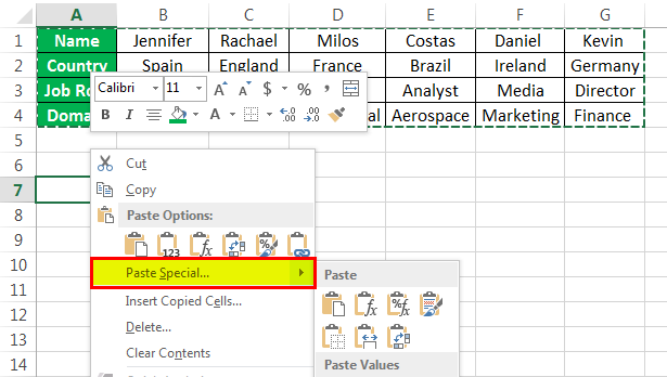
- Select a blank cell and ensure it is outside the original data range. Paste the data by pressing the “Ctrl +V” keys starting at the first blank space or cell. Then, select the down arrow from the toolbar under the “Paste” option and select “Paste Transpose.” But the easy way is to right-click the blank you chose first to paste the data. Then, select “Paste Special” from it.

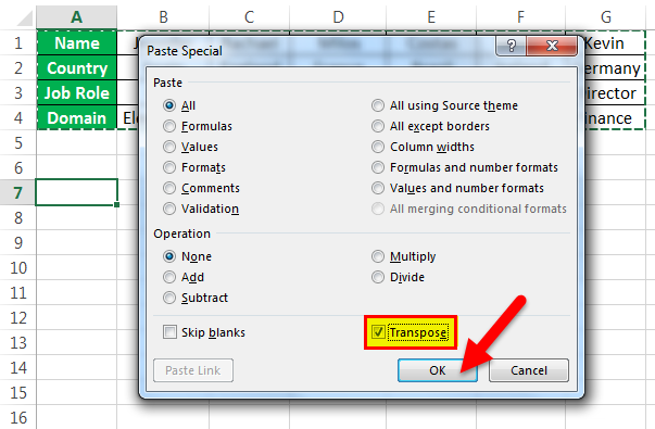
- Then, a “Paste Special” dialog box will appear from which select the “Transpose” option. And click “OK.”

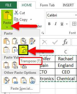
- In the above figure, copy the data which needs to be transposed and then click on the down arrow of the Paste option and form the options select Transpose. (Paste-Transpose)

It shows how the transpose function is performed to convert rows to columns.


#2 Using TRANSPOSE Formula
When a user wants to keep the same connections of the rotating table with the original table, it can use a transposing method using a formula. This method is also quicker in converting rows to columns in Excel. But, it does not keep the source formatting and links it to a transposed table.
Example
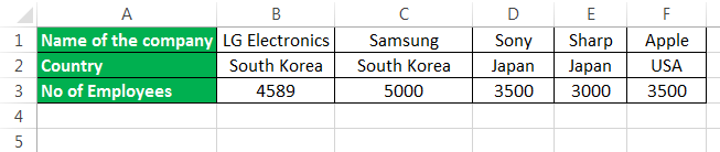
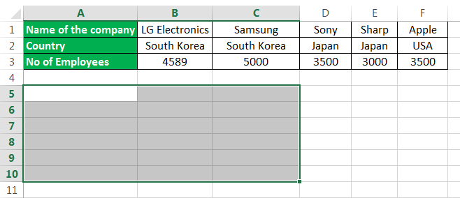
Consider the example below, as shown in figure 6, where it shows the company’s names, location, and the number of employees.
The steps to transpose rows to columns in excel using formula are as follows:
- First, count the number of rows and columns in your original excel table. And then, select the same number of blank cells but ensure you have to transpose the rows to columns to choose the blank cells in the opposite direction. Like in example 2, the number of rows is 3, and the number of columns is 6. So, you will select 6 blank rows and 3 blank columns.
- In the first empty cell, enter the TRANSPOSE formula in excelThe TRANSPOSE function in excel helps rotate (switch) the values from rows to columns and vice versa. Being a part of the Excel lookup and reference functions, its purpose is to organize the data in the desired format. To execute the formula, the exact size of the range to be transposed is selected and the CSE key (“Control+Shift+Enter”) is pressed.
read more ‘=TRANSPOSE($A$1:$F$3)’.
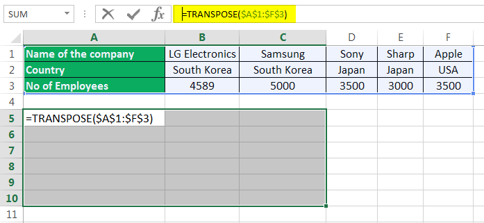
- Since this formula needs to be applied for other blank cells so press ‘Ctrl+Shift+Enter.’
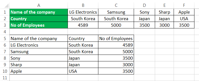
The rows are converted to columns.
Advantages
- The Paste Special method is useful when the user needs the original formatting to be continued.
- In the transpose method, by using the TRANSPOSE function, the converted table will change its data automatically, which means that whenever the user changes the data in the original table, it will automatically change the data in the transposed table, as it is linked to it.
- Converting the rows to columns in Excel sometimes helps the user to make the audience understand their data easily and so that the audience interprets it without much effort.
Disadvantages
- If the number of rows and columns increases, then the transpose method using the Paste Special options cannot perform efficiently. In this case, the “TRANSPOSE” function will be disabled when there are many rows to be converted to columns.
- The “Transpose Paste Special” option does not link the original data to the transposed data. Therefore, if you need to change the data, you must repeat all the steps.
- In the transpose method, the source formatting is not kept the same for the transposed data by using the formula.
- After converting the rows to columns in Excel using a formula, the user cannot edit the data in the transposed table as it is linked to the source data.
Things to Remember
- We can transpose rows to columns using Paste Special methods. We can link the data to the original data by selecting “Paste Link” from the “Paste Special” dialog box.
- We can also use Excel’s INDIRECT formula and ADDRESS functions in ExcelThe address function finds the cell’s address and returns an absolute value. It requires two mandatory arguments: the row number and the column number. For example, if we use =Address(1,2), the result will be $B$1.read more to convert rows to columns and vice-versa.
Recommended Articles
This article is a guide to Convert Rows to Columns in Excel. Here, we discuss switching rows to columns in Excel using the Paste Special and TRANSPOSE formula, practical examples, and a downloadable Excel template. You may learn more about Excel from the following articles: –
- Group Columns in ExcelIn Excel, grouping one or more columns together in a worksheet is referred to as group column and I t allows you to contract or expand the column.read more
- Compare Two Columns in ExcelTwo columns in excel are compared when their entries are studied for similarities and differences.read more
- Use Columns Formula in Excel
- Column Sort in Excel
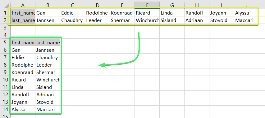
Do you have some values arranged as rows in your workbook, and do you want to convert text in rows to columns in Excel like this?
In Excel, you can do this manually or automatically in multiple ways depending on your purpose. Read on to get all the details and choose the best solution for yourself.
How to convert rows into columns or columns to rows in Excel – the basic solution
The easiest way to convert rows to columns in Excel is via the Paste Transpose option. Here is how it looks:
- Select and copy the needed range
- Right-click on a cell where you want to convert rows to columns
- Select the Paste Transpose option to rotate rows to columns
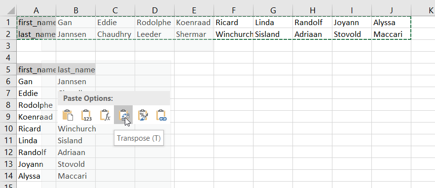
As an alternative, you can use the Paste Special option and mark Transpose using its menu.

It works the same if you need to convert columns to rows in Excel.

This is the best way for a one-time conversion of small to medium numbers of rows both in the Excel desktop and online.
Can I convert multiple rows to columns in Excel from another workbook?
The method above will work well if you want to convert rows to columns in Excel between different workbooks using Excel desktop. You need to have both spreadsheets open and do the copying and pasting as described.
However, in Excel Online, this won’t work for different workbooks. The Paste Transpose option is not available.
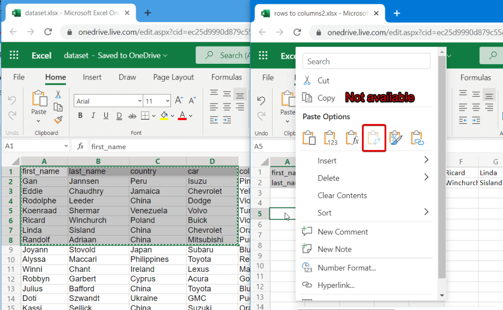
Therefore, in this case, it’s better to use the TRANSPOSE function.
How to switch rows and columns in Excel in more efficient ways
To switch rows and columns in Excel automatically or dynamically, you can use one of these options:
- Excel TRANSPOSE function
- VBA macro
- Power Query
Let’s check out each of them in the example of a data range that we imported to Excel from a Google Sheets file using Coupler.io.

Coupler.io is an integration solution that synchronizes data between source and destination apps on a regular schedule. For example, you can set up an automatic data export from Google Sheets every day to your Excel workbook.
Check out all the available Excel integrations.

How to change row to column in Excel with TRANSPOSE
TRANSPOSE is the Excel function that allows you to switch rows and columns in Excel. Here is its syntax:
=TRANSPOSE(array)array– an array of columns or rows to transpose
One of the main benefits of TRANSPOSE is that it links the converted columns/rows with the source rows/columns. So, if the values in the rows change, the same changes will be made in the converted columns.
TRANSPOSE formula to convert multiple rows to columns in Excel desktop
TRANSPOSE is an array formula, which means that you’ll need to select a number of cells in the columns that correspond to the number of cells in the rows to be converted and press Ctrl+Shift+Enter.
=TRANSPOSE(A1:J2)
Fortunately, you don’t have to go through this procedure in Excel Online.
TRANSPOSE formula to rotate row to column in Excel Online
You can simply insert your TRANSPOSE formula in a cell and hit enter. The rows will be rotated to columns right away without any additional button combinations.
Excel TRANSPOSE multiple rows in a group to columns between different workbooks
We promised to demonstrate how you can use TRANSPOSE to rotate rows to columns between different workbooks. In Excel Online, you need to do the following:
- Copy a range of columns to rotate from one spreadsheet and paste it as a link to another spreadsheet.

- We need this URL path to use in the TRANSPOSE formula, so copy it.

- The URL path above is for a cell, not for an array. So, you’ll need to slightly update it to an array to use in your TRANSPOSE formula. Here is what it should look like:
=TRANSPOSE('https://d.docs.live.net/ec25d9990d879c55/Docs/Convert rows to columns/[dataset.xlsx]dataset'!A1:D12)

You can follow the same logic for rotating rows to columns between workbooks in Excel desktop.
Are there other formulas to convert columns to rows in Excel?
TRANSPOSE is not the only function you can use to change rows to columns in Excel. A combination of INDIRECT and ADDRESS functions can be considered as an alternative, but the flow to convert rows to columns in Excel using this formula is much trickier. Let’s check it out in the following example.
How to convert text in columns to rows in Excel using INDIRECT+ADDRESS
If you have a set of columns with the first cell A1, the following formula will allow you to convert columns to rows in Excel.
=INDIRECT(ADDRESS(COLUMN(A1),ROW(A1)))

But where are the rows, you may ask! Well, first you need to drag this formula down if you are converting multiple columns to rows. Then drag it to the right.

NOTE: This Excel formula only to convert data in columns to rows starting with A1 cell. If your columns start from another cell, check out the next section.
How to convert Excel data in columns to rows using INDIRECT+ADDRESS from other cells
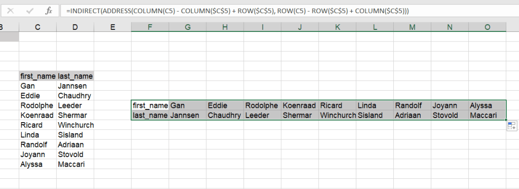
To convert columns to rows in Excel with INDIRECT+ADDRESS formulas from not A1 cell only, use the following formula:
=INDIRECT(ADDRESS(COLUMN(first_cell) - COLUMN($first_cell) + ROW($first_cell), ROW(first_cell) - ROW($first_cell) + COLUMN($first_cell)))
- first_cell – enter the first cell of your columns
Here is an example of how to convert Excel data in columns to rows:
=INDIRECT(ADDRESS(COLUMN(C5) - COLUMN($C$5) + ROW($C$5), ROW(C5) - ROW($C$5) + COLUMN($C$5)))
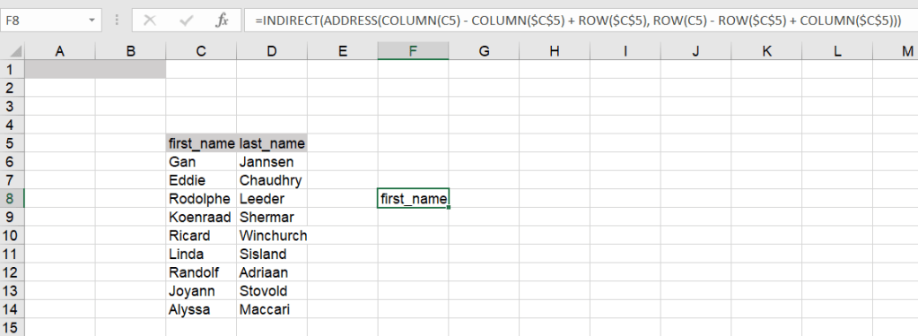
Again, you’ll need to drag the formula down and to the right to populate the rest of the cells.
How to automatically convert rows to columns in Excel VBA
VBA is a superb option if you want to customize some function or functionality. However, this option is only code-based. Below we provide a script that allows you to change rows to columns in Excel automatically.
- Go to the Visual Basic Editor (VBE). Click Alt+F11 or you can go to the Developer tab => Visual Basic.

- In VBE, go to Insert => Module.
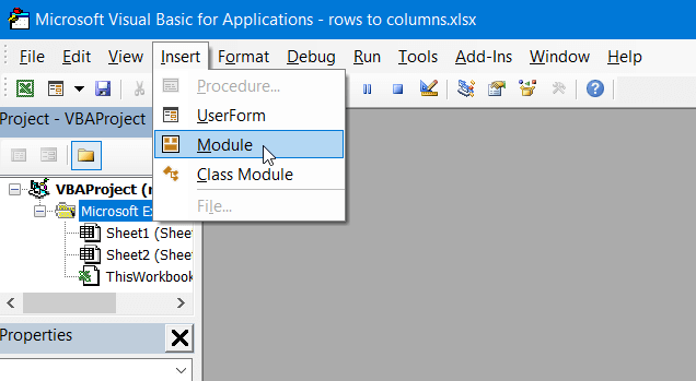
- Copy and paste the script into the window. You’ll find the script in the next section.

- Now you can close the VBE. Go to Developer => Macros and you’ll see your RowsToColumns macro. Click Run.

- You’ll be asked to select the array to rotate and the cell to insert the rotated columns.

- There you go!

VBA macro script to convert multiple rows to columns in Excel
Sub TransposeColumnsRows()
    Dim SourceRange As Range
    Dim DestRange As Range

    Set SourceRange = Application.InputBox(Prompt:="Please select the range to transpose", Title:="Transpose Rows to Columns", Type:=8)
    Set DestRange = Application.InputBox(Prompt:="Select the upper left cell of the destination range", Title:="Transpose Rows to Columns", Type:=8)

    SourceRange.Copy
    DestRange.Select
    Selection.PasteSpecial Paste:=xlPasteAll, Operation:=xlNone, SkipBlanks:=False, Transpose:=True
    Application.CutCopyMode = False

End Sub

Sub RowsToColumns()
    Dim SourceRange As Range
    Dim DestRange As Range

    Set SourceRange = Application.InputBox(Prompt:="Select the array to rotate", Title:="Convert Rows to Columns", Type:=8)
    Set DestRange = Application.InputBox(Prompt:="Select the cell to insert the rotated columns", Title:="Convert Rows to Columns", Type:=8)

    SourceRange.Copy
    DestRange.Select
    Selection.PasteSpecial Paste:=xlPasteAll, Operation:=xlNone, SkipBlanks:=False, Transpose:=True
    Application.CutCopyMode = False

End Sub
Read more in our Excel Macros Tutorial.
Convert rows to column in Excel using Power Query
Power Query is another powerful tool available for Excel users. We wrote a separate Power Query Tutorial, so feel free to check it out.
Meanwhile, you can use Power Query to transpose rows to columns. To do this, go to the Data tab, and create a query from table.

- Then select a range of cells to convert rows to columns in Excel. Click OK to open the Power Query Editor.

- In the Power Query Editor, go to the Transform tab and click Transpose. The rows will be rotated to columns.
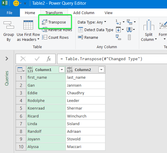
- If you want to keep the headers for your columns, click the Use First Row as Headers button.
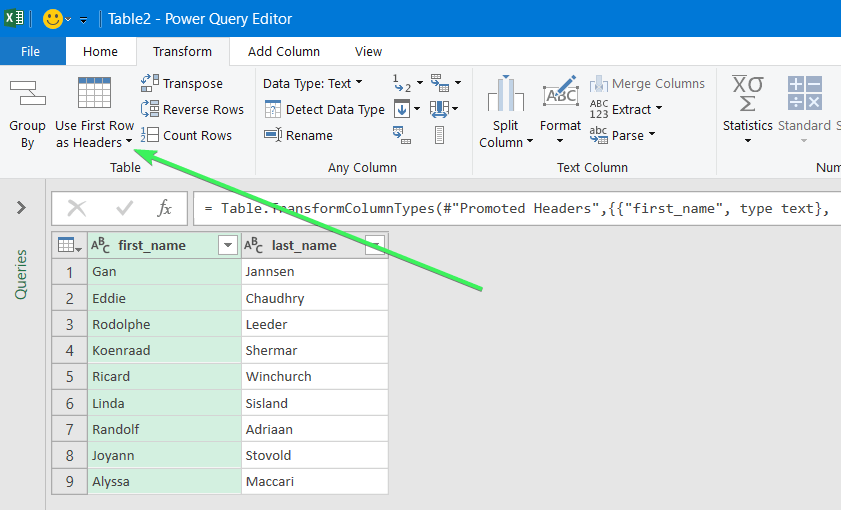
- That’s it. You can Close & Load your dataset – the rows will be converted to columns.

Error message when trying to convert rows to columns in Excel
To wrap up with converting Excel data in columns to rows, let’s review the typical error messages you can face during the flow.
Overlap error

The overlap error occurs when you’re trying to paste the transposed range into the area of the copied range. Please avoid doing this.
Wrong data type error

You may see this #VALUE! error when you implement the TRANSPOSE formula in Excel desktop without pressing Ctrl+Shift+Enter.
Other errors may be caused by typos or other misprints in the formulas you use to convert groups of data from rows to columns in Excel. Always double-check the syntax before pressing Enter or Ctrl+Shift+Enter 🙂 . Good luck with your data!
-

A content manager at Coupler.io whose key responsibility is to ensure that the readers love our content on the blog. With 5 years of experience as a wordsmith in SaaS, I know how to make texts resonate with readers’ queries✍🏼

Back to Blog
Focus on your business
goals while we take care of your data!
Try Coupler.io
Excel Rows to Columns (Table of Contents)
- Rows to Columns in Excel
- How to Convert Rows to Columns in Excel using Transpose?
Rows to Columns in Excel
In Microsoft Excel, we can change the rows to column and column to row vice versa, using TRANSPOSE. We can either use the Transpose or Transpose function to get the output.
Definition of Transpose
Transpose function normally returns a transposed range of cells which is used to switch the rows to columns and columns to rows vice versa, i.e. we can convert a vertical range of cells to a horizontal range of cells or a horizontal range of cells to a vertical range of cells in excel.
For example, a horizontal range of cells is returned if a vertical range is entered, or a vertical range of cells is returned if a horizontal range of cells is entered.
How to Convert Rows to Columns in Excel using Transpose?
It is very simple and easy. Let’s understand the working of converting rows to columns in excel by using some examples.
You can download this Convert Rows to Columns Excel?Template here – Convert Rows to Columns Excel?Template
Steps to use transpose:
- Start the cell by selecting and copying an entire range of data.
- Click on the new location.
- Right-click the cell.
- Choose to paste special, and we will find the transpose button.
- Click on the 4th option.
- We will get the result converted to rows to columns.
Example #1
Consider the below example where we have a revenue figure for sales month wise. We can see that month data are row-wise and Part number data are column-wise.
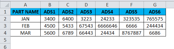
If we want to convert the rows to the column in excel, we can use the transpose function and apply it by following the below steps.
- First, select the entire cells from A To G, which has data information.
- Copy the entire data by pressing the Ctrl+ C Key.
- Now select the new cells where exactly you need to have the data.
- Right, click on the new cell, and we will get the below option which is shown below.

- Choose the option paste special.
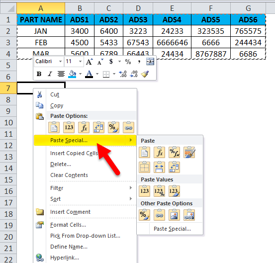
- Select the fourth option in paste special, which is called transpose, as shown in the below screenshot highlighted in yellow color.
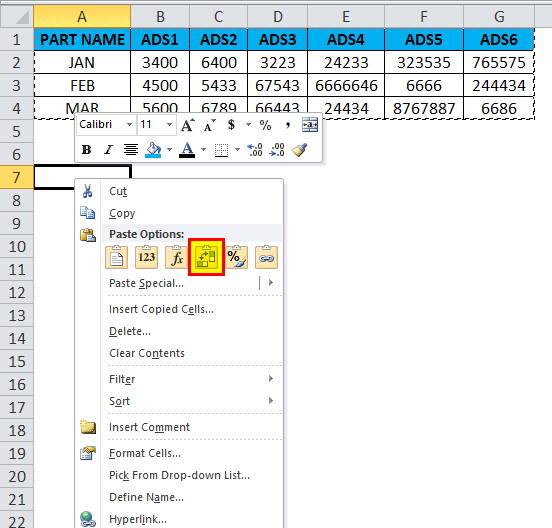
- Once we click on transpose, we will get the below output as follows.
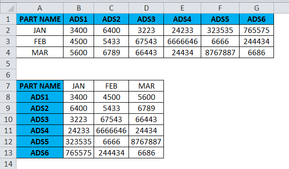
In the above screenshot, we can see that rows have been changed to column and column has been changed to rows in excel. In this way, we can easily convert the given data from row to column and column to row in excel. For the end-user, if there is a huge data, this transpose will be very useful, and it saves a lot of time instead of typing it, and we can avoid duplication.
Example #2
In this example, we will convert rows to the column in excel and see how to use transpose the employee salary data by following the below steps.
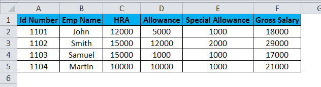
Consider the above screenshot, which has id number, emp name, HRA, Allowance, and Special Allowance. Suppose we need to convert the data column to rows; in these cases TRANSPOSE function will be very useful to convert it, which saves time instead of entering the data. We will see how to convert the column to row with the below steps.
- Click on the cell and copy the entire range of data as shown below.
- Once you copy the data, choose the new cell location.
- Right-click on the cell.
- We will get the paste special dialogue box.
- Choose Paste Special option.
- Select the Transpose option in that, as shown below.
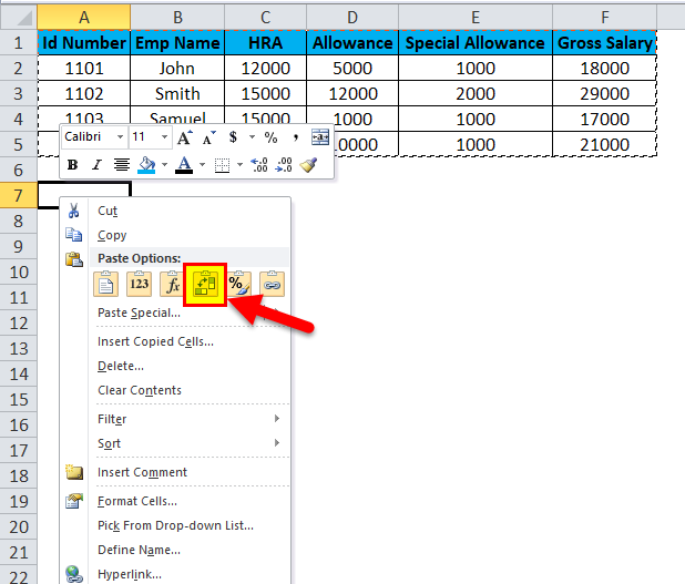
- Once you have chosen the transpose option, the excel row data will be converted to the column as shown in the below result.
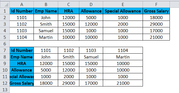
In the above screenshot, we can see the difference that row has been converted to columns; in this way, we can easily use the transpose to convert horizontal to vertical and vertical to horizontal in excel.
Transpose Function
In excel, a built-in function called Transpose Function converts rows to columns and vice versa; this function works the same as transpose. i.e. we can convert rows to columns or columns into rows vice versa.
Syntax of Transpose Function:
Argument
- Array: The range of cells to transpose.
When a set of an array is transposed, the first row is used as the first column of an array, and in the same way, the second row is used as the second column of a new one and the third row is used as the third column of the array.
If we are using the transpose function formula as an array, then we have CTRL+SHIFT +ENTER to apply it.
Example #3
In this example, we are going to see how to use the transpose function with an array with the below example.
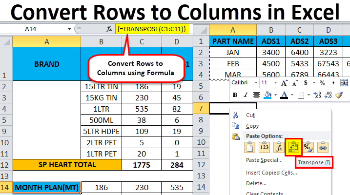
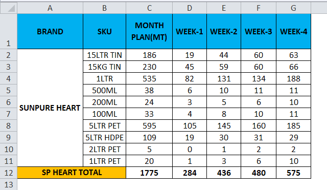
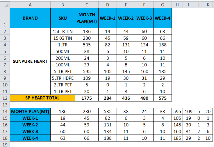
Consider the below example, which shows sales data week wise where we are going to convert the data to columns to row and row to column vice versa by using the transpose function.
- Click on the new cell.
- Select the row you want to transpose.
- Here we are going to convert the MONTH PLAN to the column.
- We can see that there are 11 rows, so in order to use the transpose function, the rows and columns should be in equal cells; if we have 11 rows, then the transpose function needs the same 11 columns to convert it.
- Choose exactly 11 columns, use the Transpose Formula, and select an array from C1 to C11, as shown in the below screenshot.
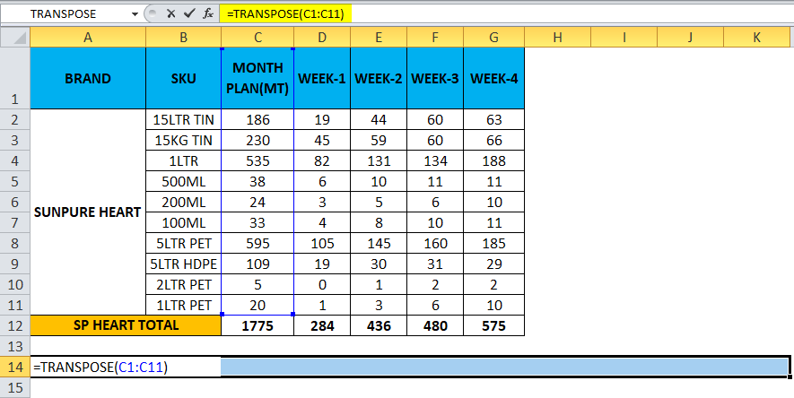
- Now use CTRL+SHIFT +ENTER to apply as an array formula.
- Once we use the CTRL+SHIFT +ENTER, we can see the open and close parenthesis in the formulation.
- We will get the output where a row has been changed to the column, which is shown below.
- Use the formula for the entire cells so that we will get the exact result.
So the Final Output will be as below.
Things to Remember about Convert Rows to Columns in Excel
- Transpose function is one of the most useful functions in excel where we can rotate the data, and the data information will not be changed while converting.
- If there are any blank or empty cells, transpose will not work, and it will give the result as zero.
- While using the array formula in transpose function, we cannot delete or edit the cells because all the data are connected with links, and Excel will throw an error message that “YOU CAN NOT CHANGE PART OF AN ARRAY.”
Recommended Articles
This has been a guide to Rows to Columns in Excel. Here we discuss how to convert rows to columns in excel using transpose along with practical examples and a downloadable excel template. Transpose can help everyone to convert multiple rows to a column in excel easily quickly. You can also go through our other suggested articles –
- Excel COLUMNS Function
- Excel ROW Function
- Unhide Columns in Excel
- Excel Rows and Columns
Creating new tables, reports and pricelists of different types, we cannot predict the number of necessary rows and columns. Using Excel program implies to a great extent creating and setting up spreadsheets, which requires inserting and deleting different elements.
First, let’s consider the methods of inserting sheet rows and columns when creating spreadsheets.
Note that in this tutorial we indicate hot keys for adding or deleting rows and columns. They should be used after highlighting the whole row or column. To highlight the row where the cursor is placed, press the combination of hot keys: SHIFT+SPACEBAR. Hot keys for highlighting a column are CTRL+SPACEBAR.
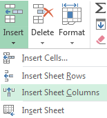
How to insert a column between other columns?
Assuming you have a pricelist lacking line item numbering:
To insert a column between other columns for filling in pricelist items numbering you can use one of the two ways:
- Move the cursor to activate A1 cell. Then go to tab «HOME», tool section «Cells» and click «Insert», in the popup menu select «Insert Sheet Columns» option.
- Right-click the heading of column A. Select «Insert» option on the shortcut menu.
- Select the column, and press the hotkey combination CTRL+SHIFT+PLUS.
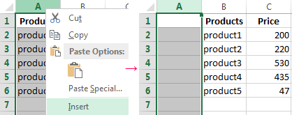
Now you can type the numbers of pricelist line items.
Simultaneous insertion of several columns
The pricelist still lacks two columns: quantity and units (items, kilograms, liters, packs). To add simultaneously, highlight the two-cell range (C1:D1). Then use the same tool on the «Insert»-«Insert Sheet Columns» main tab.
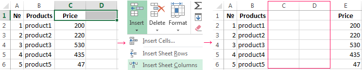
Alternatively, highlight two headings of columns C and D, right-click and select «Insert» option.
Note. Columns are always added to the left side. There appear as many new columns as many old ones have been highlighted. The order of inserted also depends on the order of highlighting. For example, next but one etc.
How to insert a row between rows in Excel?
Now let’s add a heading and a new goods line item «All for the garden» to the pricelist. To this end, let’s insert two new rows simultaneously.
Highlight the nonadjacent range of two cells A1,A4 (note that character “,” is used instead of character “:” – it means that two nonadjacent ranges should be highlighted; to make sure, type A1; A4 in the name field and press Enter). You know from the previous tutorials how to highlight nonadjacent ranges.
Now once again use the tool «HOME»-«Insert»-«Insert Sheet Columns». The picture shows how to insert a blank row between other rows in Excel.
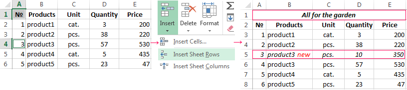
It is easy to guess the second way. You need to highlight headings of rows 1 and 3, right-click on one of the highlighted rows and select «Insert» option.
To add a row or a column in Excel use hot keys CTRL+SHIFT+PLUS having highlighted the appropriate row or column.
Note. New rows are always added above the highlighted rows.
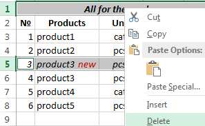
Deleting rows and columns
When working with Excel you need to delete rows and columns as often as to insert them. Therefore, you have to practice.
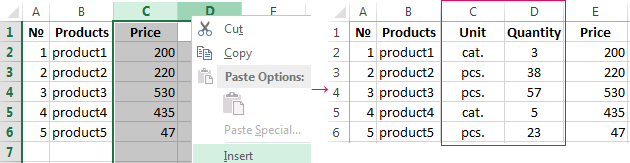
By way of illustration, let’s delete from our pricelist the numbering of goods line items and the unit column simultaneously.
Highlight the nonadjacent range of cells A1; D1 and select «HOME»-«Delete»-«Delete Sheet Rows». The shortcut menu can also be used for deleting if you highlight headings A1 and D1 instead of cells.
Row deleting is performed in the similar way. You only need to select a tool in the appropriate menu. Applying a shortcut menu is the same. You only have to highlight the rows correspondingly by row numbers.
To delete a row or a column in Excel, use hot keys CTRL+MINUS having preliminary highlighted them.
Note. Inserting new columns and rows is in fact substitution, as the number of rows (1 048 576) and columns (16 384) doesn’t change. The new just replace the old ones. You should consider this fact when filling in the sheet with data by more than 50% — 80%.
In this Article
- Insert a Single Row or Column
- Insert New Row
- Insert New Column
- Insert Multiple Rows or Columns
- Insert Multiple Rows
- Insert Multiple Columns
- Insert – Shift & CopyOrigin
- Other Insert Examples
- Insert Copied Rows or Columns
- Insert Rows Based on Cell Value
- Delete Rows or Columns
This tutorial will demonstrate how to use VBA to insert rows and columns in Excel.
To insert rows or columns we will use the Insert Method.
Insert a Single Row or Column
Insert New Row
To insert a single row, you can use the Rows Object:
Rows(4).InsertOr you can use the Range Object along with EntireRow:
Range("b4").EntireRow.InsertInsert New Column
Similar to inserting rows, we can use the Columns Object to insert a column:
Columns(4).InsertOr the Range Object, along with EntireColumn:
Range("b4").EntireColumn.InsertInsert Multiple Rows or Columns
Insert Multiple Rows
When inserting multiple rows with the Rows Object, you must enter the rows in quotations:
Rows("4:6").InsertInserting multiple rows with the Range Object works the same as with a single row:
Range("b4:b6").EntireRow.InsertInsert Multiple Columns
When inserting multiple columns with the Columns Object, enter the column letters in quotations:
Columns("B:D").InsertInserting multiple columns with the Range Object works the same as with a single column:
Range("b4:d4").EntireColumn.InsertVBA Coding Made Easy
Stop searching for VBA code online. Learn more about AutoMacro — A VBA Code Builder that allows beginners to code procedures from scratch with minimal coding knowledge and with many time-saving features for all users!

Learn More
Insert – Shift & CopyOrigin
The Insert Method has two optional arguments:
- Shift – Which direction to shift the cells
- CopyOrigin – Which cell formatting to copy (above, below, left, or right)
The Shift argument is irrelevant when inserting entire rows or columns. It only allows you to indicate to shift down or shift to the right:
- xlShiftDown – Shift cells down
- xlShiftToRight – Shift cells to the right
As you can see, you can’t shift up or to the left.
The CopyOrigin argument has two potential inputs:
- xlFormatFromLeftorAbove – (0) Newly-inserted cells take formatting from cells above or to the left
- xlFormatFromRightorBelow (1) Newly-inserted cells take formatting from cells below or to the right.
Let’s look at some examples of the CopyOrigin argument. Here’s our initial data:
This example will insert a row, taking the formatting from the above row.
Rows(5).Insert , xlFormatFromLeftOrAbove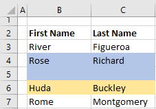
This example will insert a row, taking the formatting from the below row.
Rows(5).Insert , xlFormatFromRightOrBelow
Other Insert Examples
Insert Copied Rows or Columns
If you’d like to insert a copied row, you would use code like this:
Range("1:1").Copy
Range("5:5").Insert
Here we copy Row 1 and Insert it at Row 5.
VBA Programming | Code Generator does work for you!
Insert Rows Based on Cell Value
This will loop through a range, inserting rows based on cell values:
Sub InsertRowswithSpecificValue()

Dim cell As Range

For Each cell In Range("b2:b20")
    If cell.Value = "insert" Then
        cell.Offset(1).EntireRow.Insert
    End If
Next cell

End Sub
Delete Rows or Columns
To delete rows or columns, simply use the Delete method.
Rows(1).Delete

Range("a1").EntireRow.Delete

Columns(1).Delete

Range("a1").EntireColumn.DeleteThis post will guide you how to transpose data from rows to column with a formula in excel using both a VBA code and a formula. How do I transpose every N rows from one column to multiple columns in Excel.
In Excel, Transposing data is a common task, but when you want to transpose every N rows of data into multiple columns, it can be a bit trickier. In this post, we’ll show you how to use a VBA code and a formula to accomplish this task easily.
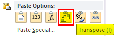
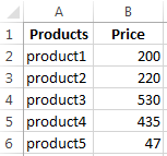
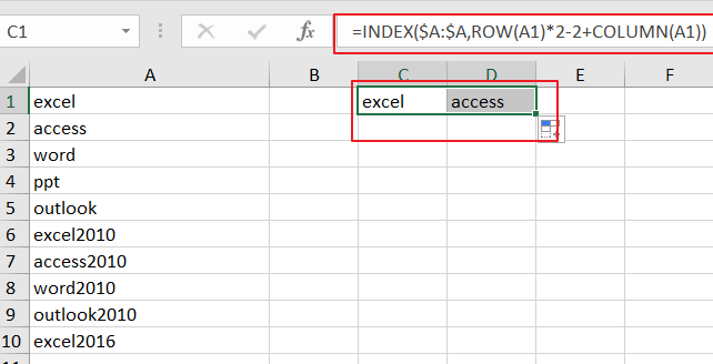
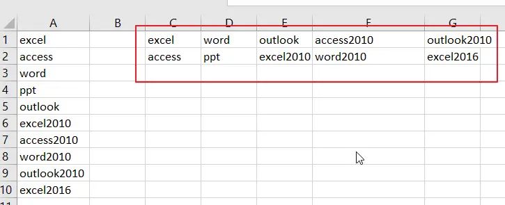
Assuming that you have a list of data in range A1:A10 in column A, and you want to transpose every 2 rows from column A to Mulitple columns. for example, you want to transpose range A1:A2 to C1:D1, A3:A4 to C2:D2. How to do it.
![]()
Table of Contents
- 1. Video: transpose Every N Rows of Data into Multiple Columns
- 2. Transpose Every N Rows of Data into Multiple Columns Using Excel Formula
- 3. Transpose Every N Rows of Data into Multiple Columns with VBA Code
- 4. Conclusion
- 5. Related Functions
1. Video: transpose Every N Rows of Data into Multiple Columns
Here’s a video tutorial on how to transpose every N rows of data into multiple columns in Excel using a formula and VBA code.
2. Transpose Every N Rows of Data into Multiple Columns Using Excel Formula
You can also transpose every N rows of data into multiple columns in Excel using a formula based on the INDEX function, the Row function and the Column Function. Like as below:
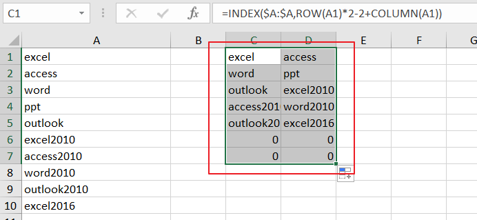
=INDEX($A:$A,ROW(A1)*2-2+COLUMN(A1))Type this formula into cell C1, and press Enter key on your keyboard, and then drag the AutoFill Handle to CEll D1.
Then you need to drag the AutoFill Handle in cell D1 down to other cells until value 0 is displayed in cells.
3. Transpose Every N Rows of Data into Multiple Columns with VBA Code
You can also use VBA code to transpose every N rows of data into multiple columns in Excel. Here’s a step-by-step guide:
Step1: Open the Excel workbook you want to work with and press “Alt + F11” to open the Visual Basic Editor.
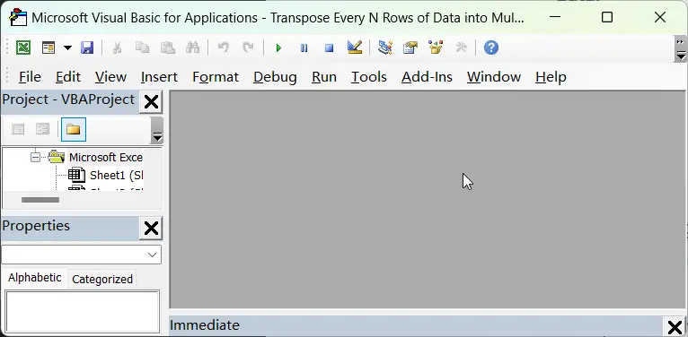
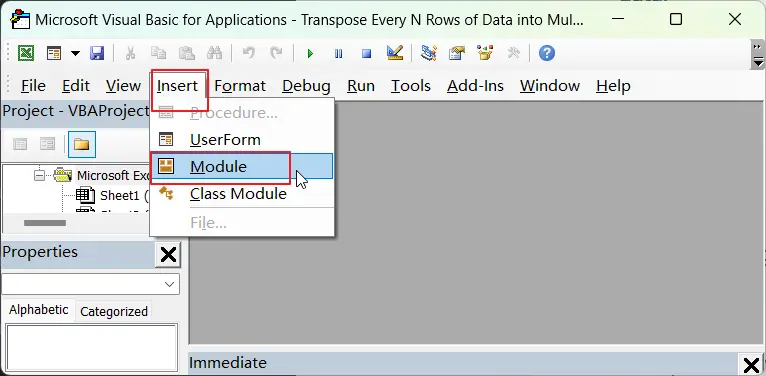
Step2: In the Visual Basic Editor, click on “Insert” from the menu bar and select “Module” to create a new module.
Step3: Copy and paste the following code into the module window.
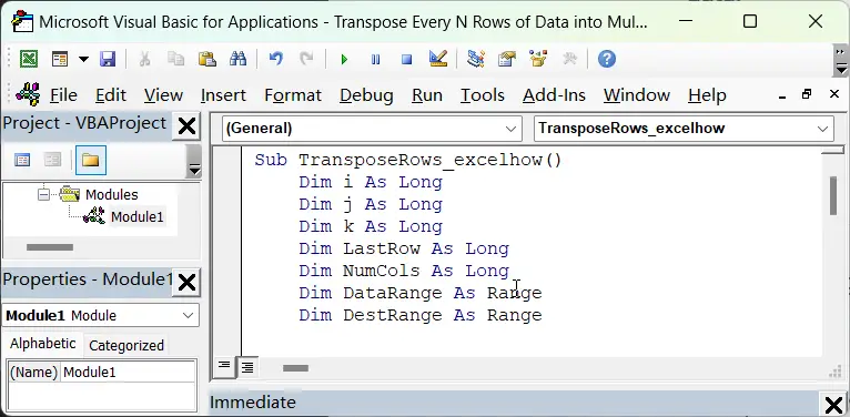
Sub TransposeRows_excelhow()
    Dim i As Long
    Dim j As Long
    Dim k As Long
    Dim LastRow As Long
    Dim NumCols As Long
    Dim DataRange As Range
    Dim DestRange As Range

    ' Set the number of rows to transpose into each column
    NumCols = Application.InputBox("Enter the number of rows to transpose into each column:")

    ' Select the range of cells to transpose
    On Error Resume Next
    Set DataRange = Application.InputBox("Select the range of cells to transpose:", Type:=8)
    On Error GoTo 0
    If DataRange Is Nothing Then Exit Sub

    ' Select the destination range for the transposed data
    On Error Resume Next
    Set DestRange = Application.InputBox("Select the destination range for the transposed data:", Type:=8)
    On Error GoTo 0
    If DestRange Is Nothing Then Exit Sub

    LastRow = DataRange.Rows.Count
    k = 0

    For i = 1 To LastRow Step NumCols
        k = k + 1
        For j = 0 To NumCols - 1
            DestRange.Offset(j, k - 1).Value = DataRange.Offset(i + j - 1, 0).Value
        Next j
    Next i
End Sub
Step4: Press “F5” or click on the “Run” button in the toolbar to run the code.
Step5: Enter the number of rows to transpose into each column, such as: 2,Click OK button.
![]()
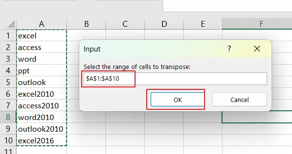
Step6: Select the range of cells to transpose, such as: selecting range A1:A10. Click OK button.
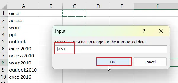
Step7: Select the destination range for the transposed data, such as: Cell C1. Click on Ok button.
Step8: Once you have entered the required information, the selected range of cells will be transposed into multiple columns according to the number of rows you specified.
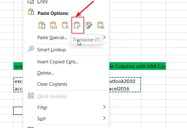
Step9: select the transposed data and press Ctrl +C to copy it. Then right click on a black cell and select “Transpose” from the Paste option menu list.
Step10: You can quickly and easily transpose every N rows of data into multiple columns using the TRANSPOSE function in Excel.
![]()
4. Conclusion
Transposing every N rows of data into multiple columns in Excel can be done using either a VBA code or a formula. Both the VBA code and the formula are effective methods for transposing every N rows of data into multiple columns in Excel. The best method to use will depend on the specific needs of your project and your level of comfort with coding in VBA.
- Excel INDEX function
The Excel INDEX function returns a value from a table based on the index (row number and column number)The INDEX function is a build-in function in Microsoft Excel and it is categorized as a Lookup and Reference Function.The syntax of the INDEX function is as below:= INDEX (array, row_num,[column_num])… - Excel ROW function
The Excel ROW function returns the row number of a cell reference.The ROW function is a build-in function in Microsoft Excel and it is categorized as a Lookup and Reference Function.The syntax of the ROW function is as below:= ROW ([reference])…. - Excel COLUMN function
The Excel COLUMN function returns the first column number of the given cell reference.The syntax of the COLUMN function is as below:=COLUMN ([reference])….
In Excel one can easily convert data columns to rows or multiple data rows to columns which is technically named transpose.
What is Transpose?
In Excel switching or rotating columns to rows or rows to columns is called Transposing the data.
And this actually shifts the dimensions of data and along with it definitely the address of different data bits will also change. Therefore, if you are into transposing your data, do it with caution as if you shift the data the dependent cells might miscalculate the figures.
Love reading about Excel? Subscribe my youtube channel dedicated to Excel.
[vc_btn title=”Subscribe” style=”custom” custom_background=”#ff0000″ custom_text=”#ffffff” size=”lg” align=”right” i_icon_fontawesome=”fa fa-youtube-play” add_icon=”true” link=”url:https%3A%2F%2Fgoo.gl%2Fx16inH||target:%20_blank|”]
Many already know how to do this. But for those who don’t this one minute Excel tutorial is for them. By the way, yes! you can use pivot tables to shift rows as columns. To learn how to make pivot tables read this readers’ favourite tutorial. And most probably you will figure out the way how rows are shifted as columns using pivot tables.
We have several ways to switch or rotate Excel data columns to rows or vice versa to accomplish this task. Following are the transpose methods we are discussing today in which few involve converting columns to rows using Excel formulas:
- Use Paste Special
- Use TRANSPOSE function
- Use INDIRECT function
- Use INDEX function
- Use Paste Special + Common Sense
Method 1: Convert columns to rows using Paste Special
Copying and Pasting is one great thing happened to PC. With Paste Special it really went miles ahead. In Excel you can copy a data and then using paste special functionality you can twist, rotate, manipulate, process and do other things with the data very easily including Transpose i.e. flipping columns to rows or rows to columns. To do this following steps will help:
Step 1: Select the data that you want to transpose and copy it using the copy button or with Ctrl+C shortcut.
Step 2: Go to the cell where you want the data to paste. And go to Home tab > clip board group > click the drop down button just under paste button > select:
- under paste sub-group click transpose button that comes with this icon; OR
- Select paste special. This will open the paste special dialogue from which check the transpose checkbox and click OK button
Your data will be transposed instantly. Told ya! it is easy!
Method 2: TRANSPOSE Function to switch columns to rows or vice versa
Yes there is a function that can do the somersault called TRANSPOSE. The use of this function is a little tricky and requires knowing more than pressing TAB so follow the steps closely.
IMPORTANT: Determine the rows and columns of your data. For example you have 2 columns and 7 rows. Once you transpose the data it will be 2 rows and 7 columns.
Step 1: Determine the rows and columns of data. In our case it is 7 rows and 2 columns
Step 2: Select a vacant region in the worksheet which is 2 rows deep and 7 columns wide.
Step 3: Press F2 key to enter edit mode while the region still selected.
Step 4: Write TRANSPOSE function following the equal sign and enter the data range that you want to transpose
Step 5: Hit CTRL+SHIFT+ENTER. Yes! Not just Enter key but Ctrl+Shift+Enter as this is an array formula
TANGO! Your data is transposed!
Benefit of TRANSPOSE Function
The best thing with using TRANSPOSE function is that if you change the values in the source range then transposed range will also change accordingly. So basically it is a live-transposed-range of the source-range.
But as this is an array function this is very much dependent on the source and if you try to change anything this tends to break. Therefore, even if it is good for many reasons, it is hard go by in many situations. So follow along to learn some more easier to go tricks to get the data transposed in Excel.
Method 3: TRANSPOSE Using INDIRECT function
INDIRECT function was introduced in one of my favourite article some time back in which we learned how to build a reference to worksheet based on cell value. I must confess that I used to think INDIRECT has very little use but this little function can prove tremendous help.
Today we will look at another use of INDIRECT function i.e. to transpose the data. However, if you use this function the treatment for column to row shift is a little different from row to column shift. So I will explain both one by one.
Transpose – Column to Row using INDIRECT
Suppose our data is based on 2 columns A and B and 7 rows from 1 to 7.
The data of column A has address like A1, A2, A3,…. A7. In this A is constant whereas due to additional rows we have increasing numbers from 1 to 7. If you understand up to this, you will understand what we are about to learn.
Lets say you want to put the transposed data starting at cell C10. I will put this formula in cell C10 and press Enter key:
=INDIRECT(“A”&COLUMN()-2)
And this formula in C11 and press Enter:
=INDIRECT(“B”&COLUMN()-2)
Now select these two cells and drag the fill handle across to column I. So there you have the data transposed. But lets understand what formula is actually doing.
Understanding INDIRECT approach to TRANSPOSE
As told earlier Indirect formula helps in converting text strings to cell references. COLUMN function actually gives us the number of column in which the formula is entered. For example if you put =COLUMN in any cell of column A it will give the value of 1 as it is first column. Similarly if you put the COLUMN function in any cell of column I, it will return 9 as it is 9th column.
So with the column function we were able to incremental numbers as we drag the formula across columns. But as we inserted the formula in third column and the not first column so it would have returned 3 in which case the first address to be fetched would have been A3. But we want the values from first cell of column A therefore we had to insert “-2”. This way we got 1, 2, 3 and not 3, 4, 5
So the formula: =INDIRECT(“A”&COLUMN()-2)
In the above formula “A” is provided as text string which is joined (concatenated) using “&” with the values generated through COLUMN function. And thus successfully built the cell references.
Now if you change the values in source range the transposed range will also change. But it is much more flexible as it won’t break if you change one item in transposed range manually.
Transpose – Rows to Columns using INDIRECT
Using the same technique learnt above, we can transpose the data from rows to columns. But in this case you will use ROWS() function instead of COLUMNS to work correctly.
As you are converting rows to columns therefore you will be going down the rows and thus you require number increments as rows are jumped. So simply adjust the formula as per your needs and use ROW instead of COLUMN and it will do the rest for you.
No you can’t simply replace the COLUMN function with ROW function as mentioned above to convert the rows back to columns. Instead you will have to use the combination of INDIRECT, ADDRESS and ROW function.
In my case to transpose first row to column I used the formula: =INDIRECT(ADDRESS(10,ROW()-11))
Whereas to convert the second row to column I used this formula: =INDIRECT(ADDRESS(11,ROW()-11))

Method 4: TRANSPOSE using INDEX functions
Using the technique learnt to transpose columns to rows above. You can use INDEX function if building reference is difficult for you and you still have your head spinning.
INDEX function is one great addition to Excel functions and formulas repository. Lets have a look at the syntax of INDEX very briefly so that we understand how can we use it to transpose the data.
INDEX(array, row_num, [column_num])
array: the range, in our case it is the range we want to transpose
row_num: the row number. In this function we have mention row number to help it fetch the value
[column_num]: this is the optional argument. If not mentioned the column number doesn’t change and it will be the same in which function is applied. But today we need this option badly!
Transposing Rows to Columns using INDEX function
Suppose our data is arranged from cell A1 to G2. Two rows and seven columns in other words. So if we transpose the data we will have 2 columns and 7 rows.
To transpose the data arranged in a row to column go to the cell from where you want the data to start. I selected cell C6 and D6 and put theses formula:
Cell C6: =INDEX($A$1:$G$2,1,ROW()-5)
Cell D6: =INDEX($A$1:$G$2,2,ROW()-5)
Select both cells and drag the fill handle down to next six rows i.e. row 12. And you will get the data transposed from rows to columns.
Understanding the formula
Lets take some time to understand the mechanics of this formula. The formula we applied in cell C6 is as follows:
=INDEX($A$1:$G$2,1,ROW()-5)
array: [$A$1:$G$2] – this is the range that we want to transpose. The reference is made absolute so that as we drag the formula this array stays static and does not change.
row_num: [1] – this represent the first row of the data and we mentioned it so that INDEX function recognize that we want it to fetch the values only from row 1 of selected array i.e. $A$1:$G$2.
column_num: [ROW()-5] – Our data A, B, C, … G is in one row but across 7 columns. That means the address of:
- value A is first row-first column
- value B is first row-second column
- value C is first row-third column; and so on…
So as we drag the formula down, we want the formula to get the values from 1st, 2nd, 3rd, 4th, 5th, 6th and 7th column. To do this we have to tell the column number. Now one way is to mention column number manually every time we put the INDEX function in next cell so that it fetches the right value.
But to automate the process of feeding column numbers to the function, I used ROW() function as the argument of column number (column_num). And as I drag the fill handle down, the ROW function will churn out row numbers inside the formula.
ROW function gives the row number. Now as I have put the INDEX function cell C6 the ROW function will tell that ROW number is 6. But we want it to be 1 as I want to fetch the values from the first column of the selected array. That is the reason we have “-5” following ROW() inside the formula. So it reduces the numbers generated by ROW function by 5 and this it will give 1, 2, 3, … 7.
Transposing Columns to Rows using INDEX function
Once you understand how INDEX function has fetched the values in above situation. Its easy to understand how to tackle the data which is arranged in columnar form and we want it to shift in rows.
For this we will make two changes:
for row_num: now we will use COLUMN() function generate numbers so that as we drag the formula towards right the row number will get updated because we are jumping across columns and thus COLUMN function will fetch the column number. Adjust the value generated by column number by adding or subtracting constants so that you get the desired result.
for column_num: mention 1 or 2 depending on the column within the selected array from which you want the values fetched.
Example
For example my data is based in 2 columns 7 rows and is housed in column C and D starting at Row 6.
I want the data transposed in rows 13 and 14 in column F. Therefore I put these formula:
cell F13:
=INDEX($C$6:$D$12,COLUMN()-5,1)
cell F14:
=INDEX($C$6:$D$12,COLUMN()-5,2)
Select both cells and drag to the right until column L
Method 5: Paste Special + Common Sense = Paste Ultimate!
We saw TRANSPOSE function went ahead of Paste Special as it was not only able push columns as rows (transpose) but were also live as transposed range was able to update as source change. We fixed some of the TRANSPOSE nuisances through INDIRECT approach. But writing formula and then dragging the range takes time.
But can we get TRANSPOSE like result using paste special? The answer is yes!
Paste Link
To get the live feed of source range we can use Paste Special’s inhouse capability called Paste link. Paste link pastes the cell references and not the values in cell and if source data changes, the linked cell will also change.
However, for unknown reasons, if you try to transpose and paste link at the same time Excel does not allow that i.e. you can either transpose or paste link. In other words, if you click Paste Link button with transpose option checked, the moment you select transpose option the paste link button gets disabled.
To get around this misery we took help of our Agent-X named common sense. Follow along!
Step 1: Copy the range and go to any vacant space in the same worksheet.
Step 2: Hit Alt+Ctrl+V to invoke paste special dialogue box and hit the button paste link. This will paste NOT the cell values but the cell references of the range you copied.
Step 3: Select the range you just pasted and hit Ctrl+H. This will bring up the REPLACE dialogue.
Step 4: In ‘Find what’ field mention equal sign i.e. “=” (without quotes) and in replace with field mention “HS=” and hit Replace ALL button. This will actually convert the formula into text as you have just replaced the equal sign with HS=
Step 5: Copy the range again and now go to the place where you want to put the transposed range. Hit Alt+Ctrl+V to bring the paste special dialogue box. Select the Transpose option and click OK. This will effectively transpose the data.
Step 6: To revert the formulas back in place so that you get the correct values in place from the source range. Hit Ctrl+H again. This time in Find what field put HS= and in replace with mention =. Hit Replace ALL button.
Now you have the live-transposed-range of the source WITHOUT using TRANSPOSE function or similar alternatives. How cheeky was that! 😉
So how do you do the transpose? If you have new ideas or any better versions of the ideas discussed do let me know in the comment section

Even after a table is created, you can add additional rows and columns. Whether you add new cells within the current range or adjacent to the table, they will automatically be formatted to match the current table style.
Insert a Row or Column Adjacent to the Table
- Click in a blank cell next to the table.
- Type a cell value.
- Click anywhere outside the cell or press the Enter key to add the value.

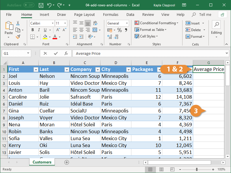
The new row or column is added to the table and the table formatting is applied.
When a formula is entered in a blank column of a table, the formula automatically fills the rest of the column, without using the AutoFill feature. If rows are added to the column, the formula appears in those rows as well.
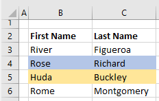
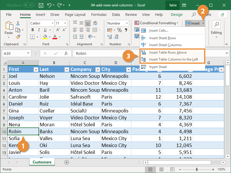
Insert a Row or Column within a Table
- Select a cell in the table row or column next to where you want to add the row or column.
Insert options aren’t available if you select a column header.
- Click the Insert list arrow on the Home tab.
- Select an insert table option.
- Insert Table Rows Above: Inserts a new row above the select cell.
- Insert Table Columns to the Left: Inserts a new column to the left of the selected cell.
Right-click a row or column next to where you want to add data, point to Insert in the menu, and select an insertion option.
Delete Rows and Columns
You can also remove unwanted table rows and columns by deleting them.
- Select a cell in the row or column you want to delete.
- Click the Delete list arrow.
- Select Delete Table Rows or Delete Table Columns.
Right-click the row or column you want to delete, point to Delete in the menu, and select Table Columns or Table Rows.
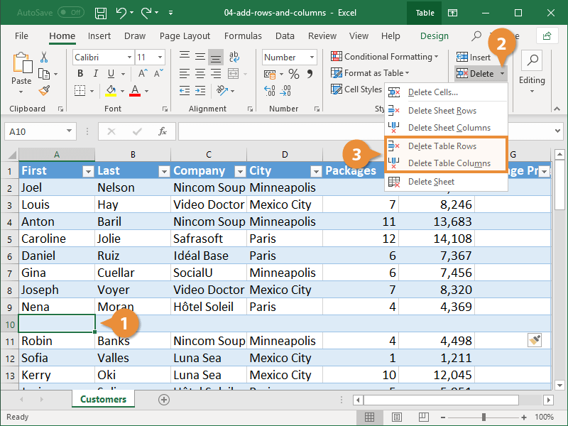
The selected row(s) or column(s) and all the data in them are deleted.

FREE Quick Reference
Click to Download
Free to distribute with our compliments; we hope you will consider our paid training.