

We all deal with multiple sheets in a single workbook, don’t we? Here is a smart way to create an Index of all your Sheets. You can click on the sheet name to navigate to that sheet.
Here is how we do it
Assume that we have 5 Sheets
![]()
And we would like to have an Index placed (in a new sheet) with the sheet names hyperlinked to the respective sheet.
It can be done with a simple VBA Code
Here comes a Code
Sub CreateIndex()
Dim sheetnum As Integer
Sheets.Add before:=Sheets(1)
For sheetnum = 2 To Worksheets.Count
 ActiveSheet.Hyperlinks.Add _
 Anchor:=Cells(sheetnum - 1, 1), _
 Address:='', _
 SubAddress:=''' & Worksheets(sheetnum).Name & ''!A1', _
 TextToDisplay:=Worksheets(sheetnum).Name
Next sheetnum
ActiveWindow.DisplayGridlines = False
End Sub
Follow the steps
- Copy this Code
- Open the excel workbook where you want to create a Sheet Index
- Press the shortcut Alt + F11 to open the Visual Basic Window
- In the Insert Menu, click on Module or use the shortcut Alt i m to add a Module. Module is the place where the code is written
- In the blank module paste the code and close the Visual Basic Editor
- Then use the shortcut Alt + F8 to open the Macro Box. You would have the list of all the macros here
- You would see the Macro that you have just pasted in the Module as ‘CreateIndex’
- Run it. You would see an Index with all the sheet names hyperlinked to the respective sheet.
Other Useful Macros
- Automated Filter with Macro
- Unhiding Multiple Sheets at Once
- Covert Numbers into Indian Currency Words
Topics that I write about…

goodly
![]()
Download Article
![]()
Download Article
If your Excel workbook contains numerous worksheets, you can add a table of contents that indexes all of your sheets with clickable hyperlinks. This tutorial will teach you how to make an index of sheet names with page numbers in your Excel workbook without complicated VBA scripting, and how to add helpful «back to index» buttons to each sheet to improve navigation.
-

1
Create an index sheet in your workbook. This sheet can be anywhere in your workbook, but you’ll usually want to place the tab at the beginning like a traditional table of contents.
- To create a new sheet, click the + at the bottom of the active worksheet. Then, right-click the new tab, select Rename, and type a name for your sheet like Index or Worksheets.
- You can rearrange sheets by dragging their tabs left or right at the bottom of your workbook.
-
2
Type Page Number into cell A1 of your index sheet. Column A is where you’ll be placing the page numbers for each sheet.
Advertisement
-
3
Type Sheet Name into cell B1 of your index sheet. This will be the column header above your list of worksheets.
-
4
Type Link into cell C1 of your index sheet. This is the column header that will appear above hyperlinks to each worksheet.
-
5
Click the Formulas tab. It’s at the top of Excel.
-
6
Click Define Name. It’s on the «Defined Names» tab at the top of Excel.
-
7
Type SheetList into the «Name» field. This names the formula you’ll be using with the INDEX function.[1]
-
8
Type the formula into the «Refers to» field and click OK. The formula is =REPLACE(GET.WORKBOOK(1),1,FIND("]",GET.WORKBOOK(1)),"").
-
9
Enter page numbers in column A. This is the only part you’ll have to do manually. For example, if your workbook has 20 pages, you’ll type 1 into A2, 2 into A3, etc., and continue numbering down until you’ve entered all 20 page numbers.
- To quickly populate the page numbers, type the first two page numbers into A2 and A3, click A3 to select it, and then drag the square at A3’s bottom-right corner down until you’ve reached the number of pages in your workbook. Then, click the small icon with a + that appears at the bottom-right corner of the column and select Fill Series.
-
10
Type this formula into cell B2 of your index sheet. The formula is =INDEX(SheetList,A2). When you press Enter or Return, you’ll see the name of the first sheet in your workbook.
-
11
Fill the rest of column B with the formula. To do this, just click B2 to select it, and then double-click the square at its bottom-right corner. This adds the name of each worksheet corresponding to the page numbers you typed into column A.
-
12
Type this formula into C2 of your worksheet. The formula is =HYPERLINK("#'"&B2&"'!A1","Go to Sheet"). When you press Enter or Return, you’ll see a hyperlink to the first page in your index called «Go to Sheet.»
-
13
Fill the rest of column C with the formula. To do this, click C2 to select it, and then double-click the square at its bottom-right corner. Now each sheet in your workbook has a clickable hyperlink that takes you right to that page.
-
14
Save your workbook in the macro-enabled format. Because you created a named range, you’ll need to save your workbook in this format.[2]
Here’s how:- Go to File > Save.
- On the pop-up message that warns you about saving a macro-free workbook, click No.
- In the «Save as type» or file format menu, select Excel Macro-Enabled Workbook (*.xlsm) and click Save.


Advertisement
-
1
Click your index or table of contents sheet. If you have a lot of pages in your workbook, it’ll be helpful to readers to add quick «Back to Index» or «Back to Table of Contents» links to each sheet so they don’t have to scroll through lots of worksheet tabs after clicking to that page. Start by opening your index sheet.
-
2
Name the index. To do this, just click the field directly above cell A1, type Index, and then press Enter or Return.
- Don’t worry if the field already contains a cell address.
-
3
Click any of the sheets in your workbook. Now you’ll create your back button. Once you create a back button on one sheet, you can just copy and paste it onto other sheets.
-
4
Click the Insert tab. It’s at the top of the screen.
-
5
Click the Illustrations menu and select Shapes. This option will be in the upper-left area of Excel.
-
6
Click a shape for your button. For example, if you want to create a back-arrow icon sort of like your web browser’s back button, you can click the left-pointing arrow under the «Block Arrows» header.
-
7
Click the location where you want to place the button. Once you click, the shape will appear. If you want, you can change the color and look using the options at the top, and/or resize the shape by dragging any of its corners.
-
8
Type some text onto the shape. The text you type should be something like «Back to Index.» You can double-click the shape to place the cursor and start typing right onto the actual shape
- You might need to drag the corner of the shape to resize it so the text fits.
- To place a text box on or near the shape before typing, just click the Shape Format menu at the top (while the shape is selected), click Text Box in the toolbar, and then click and drag a text box.
- You can stylize the text using the options in Text on the toolbar while the shape is selected.
-
9
Right-click the shape and select Link. This opens the Insert Hyperlink dialog.[3]
-
10
Click the Place in This Document icon. It’s in the left panel.
-
11
Select your index under «Defined Names» and click OK. You might have to click the + next to the column header to see the Index option. This makes the text in the shape a clickable hyperlink that takes you right to the index.
-
12
Copy and paste the hyperlink to other sheets. To do this, just right-click the shape and select Copy. Then, you can paste it onto any other page by right-clicking the desired location and selecting the first icon under «Paste Options» (the one that says «Use Destination Theme» when you hover the mouse over it).


Advertisement
Ask a Question
200 characters left
Include your email address to get a message when this question is answered.
Submit
Advertisement
Thanks for submitting a tip for review!
About This Article
Article SummaryX
To create a table of contents in Excel, you can use the «Defined Name» option to create a formula that indexes all sheet names on a single page. Then, you can use the INDEX function to list the sheet names, as well as the HYPERLINK function to create quick links to each sheet.
Did this summary help you?
Thanks to all authors for creating a page that has been read 55,649 times.
Is this article up to date?
In this post we’ll find out how to get a list of all the sheet names in the current workbook without using VBA.
This can be pretty handy if you have a large workbook with hundreds of sheets and you want to create a table of contents. This method uses the little known and often forgotten Excel 4 macro functions.
These functions aren’t like Excel’s other functions such as SUM, VLOOKUP, INDEX etc. These functions won’t work in a regular sheet, they only work in named functions and macro sheets. For this trick we’re going to use one of these in a named function.
In this example, I’ve created a workbook with a lot of sheets. There are 50 sheets in this example so I was lazy and didn’t rename them from the default names.
Now we will create our named function.
- Go to the Formulas tab.
- Press the Define Name button.
- Enter SheetNames into the name field.
- Enter the following formula into the Refers to field.
=REPLACE(GET.WORKBOOK(1),1,FIND("]",GET.WORKBOOK(1)),"") - Hit the OK button.
In a sheet within the workbook enter the numbers 1,2,3,etc… into column A starting at row 2 and then in cell B2 enter the following formula and copy and paste it down the column until you have a list of all your sheet names.
=INDEX(SheetNames,A2)As a bonus, we can also create a hyperlink so that if you click on the link it will take you to that sheet. This can be handy for navigating through a spreadsheet with lots of sheets. To do this add this formula into the column C.
= HYPERLINK ( "#'" & B2 & "'!A1", "Go To Sheet" )Note, to use this method you will need to save the file as a macro enabled workbook (.xls, .xlsm or .xlsb). Not too difficult and no VBA needed.
Video Tutorial
This video will show you two methods to list all the sheet names in a workbook.
- The first method uses a VBA procedure from this post.
- The second (skip to 3:15 in the video) uses the method in the above post.
About the Author
John is a Microsoft MVP and qualified actuary with over 15 years of experience. He has worked in a variety of industries, including insurance, ad tech, and most recently Power Platform consulting. He is a keen problem solver and has a passion for using technology to make businesses more efficient.
Summary
To list the index numbers of sheets in an Excel workbook, you can enter the sheet names, then use a formula based on the SHEET and INDIRECT functions. In the example shown, the formula in C5 is:
=SHEET(INDIRECT(B5&"!A1"))
Generic formula
=SHEET(INDIRECT(name&"!A1"))Explanation
The INDIRECT function tries to evaluate text as a valid reference. In this case, the sheet name is pulled from column B and concatenated with an exclamation point and the text A1:
=B5&"!A1"
="Sheet1"&"!A1"
="Sheet1!A1"
The INDIRECT function then coerces the text «Sheet1!A1» into a valid reference, which is passed into the SHEET function.
The SHEET function then returns the current index for each sheet as listed.

Author![]()
Dave Bruns
Hi — I’m Dave Bruns, and I run Exceljet with my wife, Lisa. Our goal is to help you work faster in Excel. We create short videos, and clear examples of formulas, functions, pivot tables, conditional formatting, and charts.
Related Information
There are hundreds and hundreds of Excel sites out there. I’ve been to many and most are an exercise in frustration. Found yours today and wanted to let you know that it might be the simplest and easiest site that will get me where I want to go.
Get Training
Quick, clean, and to the point training
Learn Excel with high quality video training. Our videos are quick, clean, and to the point, so you can learn Excel in less time, and easily review key topics when needed. Each video comes with its own practice worksheet.
View Paid Training & Bundles
Help us improve Exceljet
If you have an Excel workbook that has hundreds of worksheets, and now you want to get a list of all the worksheet names, you can refer to this article. Here we will share 3 simple methods with you.
Sometimes, you may be required to generate a list of all worksheet names in an Excel workbook. If there are only few sheets, you can just use the Method 1 to list the sheet names manually. However, in the case that the Excel workbook contains a great number of worksheets, you had better use the latter 2 methods, which are much more efficient.
Method 1: Get List Manually
- First off, open the specific Excel workbook.
- Then, double click on a sheet’s name in sheet list at the bottom.
- Next, press “Ctrl + C” to copy the name.

- Later, create a text file.
- Then, press “Ctrl + V” to paste the sheet name.

- Now, in this way, you can copy each sheet’s name to the text file one by one.


Method 2: List with Formula
- At the outset, turn to “Formulas” tab and click the “Name Manager” button.
- Next, in popup window, click “New”.

- In the subsequent dialog box, enter “ListSheets” in the “Name” field.
- Later, in the “Refers to” field, input the following formula:

=REPLACE(GET.WORKBOOK(1),1,FIND("]",GET.WORKBOOK(1)),"")

- After that, click “OK” and “Close” to save this formula.
- Next, create a new worksheet in the current workbook.
- Then, enter “1” in Cell A1 and “2” in Cell A2.
- Afterwards, select the two cells and drag them down to input 2,3,4,5, etc. in Column A.

- Later, put the following formula in Cell B1.

=INDEX(ListSheets,A1)

- At once, the first sheet name will be input in Cell B1.
- Finally, just copy the formula down until you see the “#REF!” error.


Method 3: List via Excel VBA
- For a start, trigger Excel VBA editor according to “How to Run VBA Code in Your Excel“.
- Then, put the following code into a module or project.
Sub ListSheetNamesInNewWorkbook()
    Dim objNewWorkbook As Workbook
    Dim objNewWorksheet As Worksheet

    Set objNewWorkbook = Excel.Application.Workbooks.Add
    Set objNewWorksheet = objNewWorkbook.Sheets(1)

    For i = 1 To ThisWorkbook.Sheets.Count
        objNewWorksheet.Cells(i, 1) = i
        objNewWorksheet.Cells(i, 2) = ThisWorkbook.Sheets(i).Name
    Next i

    With objNewWorksheet
         .Rows(1).Insert
         .Cells(1, 1) = "INDEX"
         .Cells(1, 1).Font.Bold = True
         .Cells(1, 2) = "NAME"
         .Cells(1, 2).Font.Bold = True
         .Columns("A:B").AutoFit
    End With
End Sub

- Later, press “F5” to run this macro right now.
- At once, a new Excel workbook will show up, in which you can see the list of worksheet names of the source Excel workbook.


Comparison
| Advantages | Disadvantages | |
| Method 1 | Easy to operate | Too troublesome if there are a lot of worksheets |
| Method 2 | Easy to operate | Demands you to type the index first |
| Method 3 | Quick and convenient | Users should beware of the external malicious macros |
| Easy even for VBA newbies |
Excel Gets Corrupted
MS Excel is known to crash from time to time, thereby damaging the current files on saving. Therefore, it’s highly recommended to get hold of an external powerful Excel repair tool, such as DataNumen Outlook Repair. It’s because that self-recovery feature in Excel is proven to fail frequently.
Author Introduction:
Shirley Zhang is a data recovery expert in DataNumen, Inc., which is the world leader in data recovery technologies, including sql fix and outlook repair software products. For more information visit www.datanumen.com
This post will guide you how to get a list of all worksheet names in an excel workbook. How do I List the Sheet names with Formula in Excel. How to generate a list of all sheet tab names using Excel VBA Code.
Assuming that you have a workbook that has hundreds of worksheets and you want to get a list of all the worksheet names in the current workbook. And the below will introduce 3 methods with you.
Table of Contents
- Get All Worksheet Names Manually
- Get All Worksheet Names with Formula
- Get All Sheet Names with Excel VBA Macro
- Related Functions
Get All Worksheet Names Manually
If there are only few worksheets in your workbook, and you can get a list of all worksheet tab names by manually. Let’s see the below steps:
#1 open your workbook
#2 double click on the sheet’s name in the sheet tab. Press Ctrl + C shortcuts in your keyboard to copy the selected sheet.
#3 create a notepad file, and then press Ctrl +V to paste the sheet name.
#4 follow the above steps 2-3 to copy&paste all worksheet names into notepad file.
Get All Worksheet Names with Formula
You can also use a formula to get a list of all worksheet names with a formula. You can create a formula based on the LOOKUP function, the CHOOSE function, the INDEX function, the MID function, the FIND function and the ROWS function. Just do the following steps:
#1 go to FORMULAS tab, click Name Manager command under Defined Names group. The Name Manager dialog will open.
#2 click New… button to create a define name, type Sheets in the Name text box, and type the formula into the Refers to text box.
=GET.WORKBOOK(1)&T(NOW())
#3 Type the following formula into a blank cell and press Enter key in your keyboard, and then drag the autofill handle over others cells to get the rest sheet names.
=LOOKUP("xxxxx",CHOOSE({1,2},"",INDEX(MID(Sheets,FIND("]",Sheets)+1,255),ROWS(A$1:A1))))
You will see that all sheet names have been listed in the cells.
Get All Sheet Names with Excel VBA Macro
You can also use an Excel VBA Macro to quickly get a list of all worksheet tab names in your workbook. Just do the following steps:
#1 open your excel workbook and then click on “Visual Basic” command under DEVELOPER Tab, or just press “ALT+F11” shortcut.

#2 then the “Visual Basic Editor” window will appear.
#3 click “Insert” ->”Module” to create a new module

#4 paste the below VBA code into the code window. Then clicking “Save” button.
Sub GetListOfAllSheets()
   Dim w As Worksheet
   Dim i As Integer
   i = 1
   Sheets("Sheet1").Range("A:A").Clear
   For Each w In Worksheets
       Sheets("Sheet1").Cells(i, 1) = w.Name
       i = i + 1
   Next w
End Sub
#5 back to the current worksheet, then run the above excel macro. Click Run button.
#6 Let’s see the result.
- Excel MID function
The Excel MID function returns a substring from a text string at the position that you specify.The syntax of the MID function is as below:= MID (text, start_num, num_chars)… - Excel LOOKUP function
The Excel LOOKUP function will search a value in a vector or array.The LOOKUP function is a build-in function in Microsoft Excel and it is categorized as a Lookup and Reference Function.The syntax of the LOOKUP function is as below:= LOOKUP (lookup_value, lookup_vector, [result_vector])… - Excel Choose Function
The Excel CHOOSE function returns a value from a list of values. The CHOOSE function is a build-in function in Microsoft Excel and it is categorized as a Lookup and Reference Function.The syntax of the CHOOSE function is as below:=CHOOSE (index_num, value1,[value2],…)… - Excel INDEX function
The Excel INDEX function returns a value from a table based on the index (row number and column number)The INDEX function is a build-in function in Microsoft Excel and it is categorized as a Lookup and Reference Function.The syntax of the INDEX function is as below:= INDEX (array, row_num,[column_num])… - Excel ROWS function
The Excel ROWS function returns the number of rows in a cell reference.The syntax of the ROWS function is as below:= ROWS(array)… - Excel FIND function
The Excel FIND function returns the position of the first text string (sub string) within another text string.The syntax of the FIND function is as below:= FIND(find_text, within_text,[start_num])
Содержание
- Create an Index of Sheets in Your Workbook
- How to create index of sheets in Excel with hyperlinks
- Code for creating an index of sheets
- Tweaks
- INDEX function
- Array form
- Description
- Syntax
- Remarks
- Examples
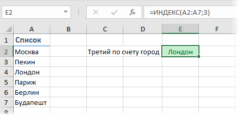
- Example 1
- Example 2
- Reference form
- Description
- Syntax
- Remarks
- Examples
- 5 вариантов использования функции ИНДЕКС (INDEX)
- Вариант 1. Извлечение данных из столбца по номеру ячейки
- Вариант 2. Извлечение данных из двумерного диапазона
- Вариант 3. Несколько таблиц
- Вариант 4. Ссылка на столбец / строку
- Вариант 5. Ссылка на ячейку
Create an Index of Sheets in Your Workbook
If you’ve spent much time in a workbook with many worksheets, you know how painful it can be to find a particular worksheet. An index sheet available to every worksheet is a navigational must-have.
Using an index sheet will enable you to quickly and easily navigate throughout your workbook so that with one click of the mouse, you will be taken exactly where you want to go, without fuss. You can create an index in a couple of ways.
You might be tempted to simply create the index by hand. Create a new worksheet, call it Index or the like, enter a list of all your worksheet’s names, and hyperlink each to the appropriate sheet by selecting Insert » Hyperlink. or by pressing Ctrl/ -K. Although this method is probably sufficient for limited instances in which you don’t have too many sheets and they won’t change often, you’ll be stuck maintaining your index by hand.
The following code will automatically create a clickable, hyperlinked index of all the sheets you have in the workbook. The index is re-created each time the sheet that houses the code is activated.
This code should live in the private module for the Sheet object. Insert a new worksheet into your workbook and name it something appropriate- Index , for instance. Right-click the index sheet’s tab and select View Code from the context menu. Enter the following Visual Basic code (Tools » Macro » Visual Basic Editor or Alt/Option-F11):
Press Alt/-Q to get back to your workbook and then save your changes. Notice that the code names (such as when you name a cell or range of cells in Excel) cell A1 on each sheet Start , plus a unique whole number representing the index number of the sheet . This ensures that A1 on each sheet has a different name. If A1 on your worksheet already has a name, you should consider changing any mention of A1 in the code to something more suitable-an unused cell anywhere on the sheet, for instance.
You should be aware that if you select File » Properties » Summary and enter a URL as a hyperlink base, the index created from the preceding code possibly will not work. A hyperlink base is a path or URL that you want to use for all hyperlinks with the same base address that are inserted in the current document.
Another, more user-friendly, way of constructing an index is to add a link to the list of sheets as a context-menu item, keeping it just a right-click away. We’ll have that link open the standard workbook tabs command bar. You generally get to this command bar by right-clicking any of the sheet tab scroll arrows on the bottom left of any worksheet, as shown in figure.
Figure. Tabs command bar displayed by right-clicking the sheet scroll tabs

To link that tab’s command bar to a right-click in any cell, enter the following code in the VBE:
Next, you’ll need to insert a standard module to house the IndexCode macro, called by the preceding code whenever the user right-clicks in a cell. It is vital that you use a standard module next, as placing the code in the same module as Workbook_SheetBeforeRightClick will mean Excel will not know where to find the macro called IndexCode .
Select Insert » Module and enter the following code:
Press Alt/-Q to get back to the Excel interface.
Now, right-click within any cell on any worksheet and you should see a new menu item called Sheet Index that will take you right to a list of sheets in the workbook.
Источник
How to create index of sheets in Excel with hyperlinks

In this guide, we’re going to show you how to create index page of worksheets in Excel with hyperlinks. Using VBA, you can automatically update the hyperlinks after adding or removing sheets.
First, you need to create a new sheet for the index.
- Create a new sheet.
- Right-click on its tab.
- Select View Code option to open VBA editor for the corresponding sheet.

Alternatively, you can press the Alt + F11 key combination to open the VBA window and select the index sheet from the left pane.
Copy the following code and paste into the editor. Once you pasted the code, it will run every time you open that worksheet.
Code for creating an index of sheets

You can close the VBA window now and test by opening another sheet other than the index sheet and then go back to the index sheet. The code automatically updates the worksheets that are not hidden.

Remember to save your file as a macro-enabled workbook (xlsm).

Tweaks
The code creates hyperlinks for visible sheets only. We added this check to hide sheets used for calculations or static data which should not be accessible to the end users.
Источник
INDEX function
The INDEX function returns a value or the reference to a value from within a table or range.

There are two ways to use the INDEX function:
If you want to return the value of a specified cell or array of cells, see Array form.
If you want to return a reference to specified cells, see Reference form.
Array form
Description
Returns the value of an element in a table or an array, selected by the row and column number indexes.
Use the array form if the first argument to INDEX is an array constant.
Syntax
INDEX(array, row_num, [column_num])
The array form of the INDEX function has the following arguments:
array Required. A range of cells or an array constant.
If array contains only one row or column, the corresponding row_num or column_num argument is optional.
If array has more than one row and more than one column, and only row_num or column_num is used, INDEX returns an array of the entire row or column in array.
row_num Required, unless column_num is present. Selects the row in array from which to return a value. If row_num is omitted, column_num is required.
column_num Optional. Selects the column in array from which to return a value. If column_num is omitted, row_num is required.
If both the row_num and column_num arguments are used, INDEX returns the value in the cell at the intersection of row_num and column_num.
row_num and column_num must point to a cell within array; otherwise, INDEX returns a #REF! error.
If you set row_num or column_num to 0 (zero), INDEX returns the array of values for the entire column or row, respectively. To use values returned as an array, enter the INDEX function as an array formula.
Note: If you have a current version of Microsoft 365, then you can input the formula in the top-left-cell of the output range, then press ENTER to confirm the formula as a dynamic array formula. Otherwise, the formula must be entered as a legacy array formula by first selecting the output range, input the formula in the top-left-cell of the output range, then press CTRL+SHIFT+ENTER to confirm it. Excel inserts curly brackets at the beginning and end of the formula for you. For more information on array formulas, see Guidelines and examples of array formulas.
Examples
Example 1
These examples use the INDEX function to find the value in the intersecting cell where a row and a column meet.
Copy the example data in the following table, and paste it in cell A1 of a new Excel worksheet. For formulas to show results, select them, press F2, and then press Enter.
Value at the intersection of the second row and second column in the range A2:B3.
Value at the intersection of the second row and first column in the range A2:B3.
Example 2
This example uses the INDEX function in an array formula to find the values in two cells specified in a 2×2 array.
Note: If you have a current version of Microsoft 365, then you can input the formula in the top-left-cell of the output range, then press ENTER to confirm the formula as a dynamic array formula. Otherwise, the formula must be entered as a legacy array formula by first selecting two blank cells, input the formula in the top-left-cell of the output range, then press CTRL+SHIFT+ENTER to confirm it. Excel inserts curly brackets at the beginning and end of the formula for you. For more information on array formulas, see Guidelines and examples of array formulas.
Value found in the first row, second column in the array. The array contains 1 and 2 in the first row and 3 and 4 in the second row.
Value found in the second row, second column in the array (same array as above).
Reference form
Description
Returns the reference of the cell at the intersection of a particular row and column. If the reference is made up of non-adjacent selections, you can pick the selection to look in.
Syntax
INDEX(reference, row_num, [column_num], [area_num])
The reference form of the INDEX function has the following arguments:
reference Required. A reference to one or more cell ranges.
If you are entering a non-adjacent range for the reference, enclose reference in parentheses.
If each area in reference contains only one row or column, the row_num or column_num argument, respectively, is optional. For example, for a single row reference, use INDEX(reference,,column_num).
row_num Required. The number of the row in reference from which to return a reference.
column_num Optional. The number of the column in reference from which to return a reference.
area_num Optional. Selects a range in reference from which to return the intersection of row_num and column_num. The first area selected or entered is numbered 1, the second is 2, and so on. If area_num is omitted, INDEX uses area 1. The areas listed here must all be located on one sheet. If you specify areas that are not on the same sheet as each other, it will cause a #VALUE! error. If you need to use ranges that are located on different sheets from each other, it is recommended that you use the array form of the INDEX function, and use another function to calculate the range that makes up the array. For example, you could use the CHOOSE function to calculate which range will be used.
For example, if Reference describes the cells (A1:B4,D1:E4,G1:H4), area_num 1 is the range A1:B4, area_num 2 is the range D1:E4, and area_num 3 is the range G1:H4.
After reference and area_num have selected a particular range, row_num and column_num select a particular cell: row_num 1 is the first row in the range, column_num 1 is the first column, and so on. The reference returned by INDEX is the intersection of row_num and column_num.
If you set row_num or column_num to 0 (zero), INDEX returns the reference for the entire column or row, respectively.
row_num, column_num, and area_num must point to a cell within reference; otherwise, INDEX returns a #REF! error. If row_num and column_num are omitted, INDEX returns the area in reference specified by area_num.
The result of the INDEX function is a reference and is interpreted as such by other formulas. Depending on the formula, the return value of INDEX may be used as a reference or as a value. For example, the formula CELL(«width»,INDEX(A1:B2,1,2)) is equivalent to CELL(«width»,B1). The CELL function uses the return value of INDEX as a cell reference. On the other hand, a formula such as 2*INDEX(A1:B2,1,2) translates the return value of INDEX into the number in cell B1.
Examples
Copy the example data in the following table, and paste it in cell A1 of a new Excel worksheet. For formulas to show results, select them, press F2, and then press Enter.
Источник
5 вариантов использования функции ИНДЕКС (INDEX)
Бывает у вас такое: смотришь на человека и думаешь «что за @#$%)(*?» А потом при близком знакомстве оказывается, что он знает пять языков, прыгает с парашютом, имеет семеро детей и черный пояс в шахматах, да и, вообще, добрейшей души человек и умница?
Так и в Microsoft Excel: есть несколько похожих функций, про которых фраза «внешность обманчива» работает на 100%. Одна из наиболее многогранных и полезных — функция ИНДЕКС (INDEX) . Далеко не все пользователи Excel про нее знают, и еще меньше используют все её возможности. Давайте разберем варианты ее применения, ибо их аж целых пять.
Вариант 1. Извлечение данных из столбца по номеру ячейки
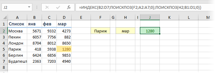
Самый простой случай использования функции ИНДЕКС – это ситуация, когда нам нужно извлечь данные из одномерного диапазона-столбца, если мы знаем порядковый номер ячейки. Синтаксис в этом случае будет:
=ИНДЕКС( Диапазон_столбец ; Порядковый_номер_ячейки )
Этот вариант известен большинству продвинутых пользователей Excel. В таком виде функция ИНДЕКС часто используется в связке с функцией ПОИСКПОЗ (MATCH) , которая выдает номер искомого значения в диапазоне. Таким образом, эта пара заменяет легендарную ВПР (VLOOKUP) :
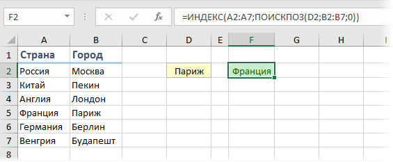
. но, в отличие от ВПР, могут извлекать значения левее поискового столбца и номер столбца-результата высчитывать не нужно.
Вариант 2. Извлечение данных из двумерного диапазона
Если диапазон двумерный, т.е. состоит из нескольких строк и столбцов, то наша функция будет использоваться немного в другом формате:
=ИНДЕКС( Диапазон ; Номер_строки ; Номер_столбца )
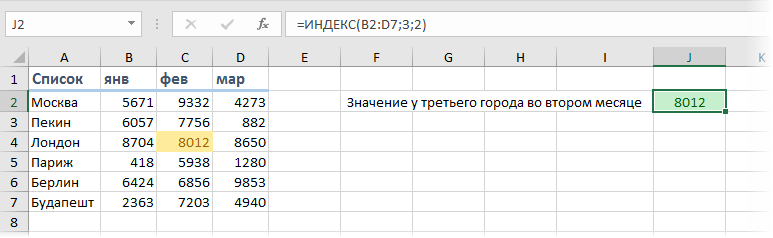
Т.е. функция извлекает значение из ячейки диапазона с пересечения строки и столбца с заданными номерами.
Легко сообразить, что с помощью такой вариации ИНДЕКС и двух функций ПОИСКПОЗ можно легко реализовать двумерный поиск:
Вариант 3. Несколько таблиц
Если таблица не одна, а их несколько, то функция ИНДЕКС может извлечь данные из нужной строки и столбца именно заданной таблицы. В этом случае используется следующий синтаксис:
=ИНДЕКС( (Диапазон1;Диапазон2;Диапазон3) ; Номер_строки ; Номер_столбца ; Номер_диапазона )
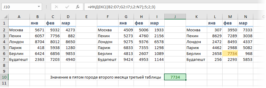
Обратите особое внимание, что в этом случае первый аргумент – список диапазонов — заключается в скобки, а сами диапазоны перечисляются через точку с запятой.
Вариант 4. Ссылка на столбец / строку
Если во втором варианте использования функции ИНДЕКС номер строки или столбца задать равным нулю (или просто не указать), то функция будет выдавать уже не значение, а ссылку на диапазон-столбец или диапазон-строку соответственно:
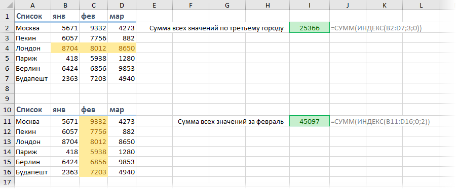
Обратите внимание, что поскольку ИНДЕКС выдает в этом варианте не конкретное значение ячейки, а ссылку на диапазон, то для подсчета потребуется заключить ее в дополнительную функцию, например СУММ (SUM) , СРЗНАЧ (AVERAGE) и т.п.
Вариант 5. Ссылка на ячейку
Общеизвестно, что стандартная ссылка на любой диапазон ячеек в Excel выглядит как Начало-Двоеточие-Конец, например A2:B5. Хитрость в том, что если взять функцию ИНДЕКС в первом или втором варианте и подставить ее после двоеточия, то наша функция будет выдавать уже не значение, а адрес, и на выходе мы получим полноценную ссылку на диапазон от начальной ячейки до той, которую нашла ИНДЕКС:
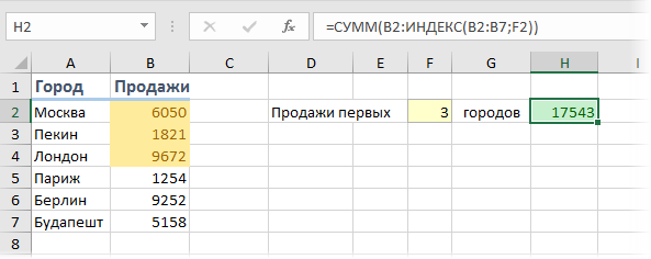
Нечто похожее можно реализовать функцией СМЕЩ (OFFSET) , но она, в отличие от ИНДЕКС, является волатильной, т.е. пересчитывается каждый раз при изменении любой ячейки листа. ИНДЕКС же работает более тонко и запускает пересчет только при изменении своих аргументов, что ощутимо ускоряет расчет в тяжелых книгах по сравнению со СМЕЩ.
Один из весьма распространенных на практике сценариев применения ИНДЕКС в таком варианте — это сочетание с функцией СЧЁТЗ (COUNTA) , чтобы получить автоматически растягивающиеся диапазоны для выпадающих списков, сводных таблиц и т.д.
Источник
If you’ve spent much time in a workbook with many worksheets, you know how painful it can be to find a particular worksheet. An index sheet available to every worksheet is a navigational must-have.
Using an index sheet will enable you to quickly and easily navigate throughout your workbook so that with one click of the mouse, you will be taken exactly where you want to go, without fuss. You can create an index in a couple of ways.
You might be tempted to simply create the index by hand. Create a new worksheet, call it Index or the like, enter a list of all your worksheet’s names, and hyperlink each to the appropriate sheet by selecting Insert » Hyperlink… or by pressing Ctrl/-K. Although this method is probably sufficient for limited instances in which you don’t have too many sheets and they won’t change often, you’ll be stuck maintaining your index by hand.
The following code will automatically create a clickable, hyperlinked index of all the sheets you have in the workbook. The index is re-created each time the sheet that houses the code is activated.
This code should live in the private module for the Sheet object. Insert a new worksheet into your workbook and name it something appropriate-Index, for instance. Right-click the index sheet’s tab and select View Code from the context menu. Enter the following Visual Basic code (Tools » Macro » Visual Basic Editor or Alt/Option-F11):
Private Sub Worksheet_Activate( )
Dim wSheet As Worksheet
Dim l As Long
l = 1
    With Me
        .Columns(1).ClearContents
        .Cells(1, 1) = "INDEX"
        .Cells(1, 1).Name = "Index"
    End With
    For Each wSheet In Worksheets
     If wSheet.Name <> Me.Name Then
      l = l + 1
      With wSheet
          .Range("A1").Name = "Start" & wSheet.Index
          .Hyperlinks.Add Anchor:=.Range("A1"), Address:="", SubAddress:= _
            "Index", TextToDisplay:="Back to Index"
      End With
         Me.Hyperlinks.Add Anchor:=Me.Cells(l, 1), Address:="",_
            SubAddress:="Start" & wSheet.Index, TextToDisplay:=wSheet.Name
     End If
    Next wSheet
End Sub
Press Alt/-Q to get back to your workbook and then save your changes. Notice that the code names (such as when you name a cell or range of cells in Excel) cell
A1 on each sheet Start, plus a unique whole number representing the index number of the sheet . This ensures that A1 on each sheet has a different name. If A1 on your worksheet already has a name, you should consider changing any mention of A1 in the code to something more suitable-an unused cell anywhere on the sheet, for instance.
You should be aware that if you select File » Properties » Summary and enter a URL as a hyperlink base, the index created from the preceding code possibly will not work. A hyperlink base is a path or URL that you want to use for all hyperlinks with the same base address that are inserted in the current document.
Another, more user-friendly, way of constructing an index is to add a link to the list of sheets as a context-menu item, keeping it just a right-click away. We’ll have that link open the standard workbook tabs command bar. You generally get to this command bar by right-clicking any of the sheet tab scroll arrows on the bottom left of any worksheet, as shown in figure.
Figure. Tabs command bar displayed by right-clicking the sheet scroll tabs
To link that tab’s command bar to a right-click in any cell, enter the following code in the VBE:
Private Sub Workbook_SheetBeforeRightClick(ByVal Sh As Object, ByVal Target
As Range, Cancel As Boolean)
Dim cCont As CommandBarButton
    On Error Resume Next
    Application.CommandBars("Cell").Controls("Sheet Index").Delete
    On Error GoTo 0
        Set cCont = Application.CommandBars("Cell").Controls.Add _
                        (Type:=msoControlButton, Temporary:=True)
        With cCont
                  .Caption = "Sheet Index"
             .OnAction = "IndexCode"
            End With
End Sub
Next, you’ll need to insert a standard module to house the IndexCode macro, called by the preceding code whenever the user right-clicks in a cell. It is vital that you use a standard module next, as placing the code in the same module as Workbook_SheetBeforeRightClick will mean Excel will not know where to find the macro called IndexCode.
Select Insert » Module and enter the following code:
Sub IndexCode( )
 Application.CommandBars("workbook Tabs").ShowPopup
End Sub
Press Alt/-Q to get back to the Excel interface.
Now, right-click within any cell on any worksheet and you should see a new menu item called Sheet Index that will take you right to a list of sheets in the workbook.
by updated Aug 01, 2016
|
Limos Пользователь Сообщений: 102 |
#1 05.07.2017 14:56:55 Добрый день! Подскажите как правильно получить следующую информацию.
Звездочка означает, что неважно какие символы будут дальше. Заранее спасибо. |
||
|
vikttur Пользователь Сообщений: 47199 |
В цикле проверяйте наличие фрагмента в имени листа. |
|
Limos Пользователь Сообщений: 102 |
Каким образом, подскажите приблизительно. |
|
_Boroda_  Пользователь Сообщений: 1496 Контакты см. в профиле |
#4 05.07.2017 15:15:03 Приблизительно так
Изменено: _Boroda_ — 05.07.2017 15:15:11 Скажи мне, кудесник, любимец ба’гов… |
||
|
vikttur Пользователь Сообщений: 47199 |
#5 05.07.2017 15:17:45
|
||
|
Limos Пользователь Сообщений: 102 |
#6 05.07.2017 15:34:42 Спасибо большое) Я это находил чтобы обновить источник данных для сводной таблицы, вот код
Но, гад выдает ошибку Run-time error ’91’ Object variable or With block variable not set Изменено: Limos — 05.07.2017 15:46:01 |
||